Simulation with Modifications to Parameters and Model Code
Simone Cassani, Philip Delff
July 13, 2026 using NMsim 0.2.7.901
Source:vignettes/NMsim-modify-model.Rmd
NMsim-modify-model.RmdIntroduction
The introduction examples and the other examples show how to perform
various types of simulations, such as typical subject simulations,
simulations of new subjects, simulation of known subjects, and
simulation with parameter uncertainty. As different as these simulations
may be, they are all simulations of a model, exactly as specified or
exactly as estimated. The examples in this document focus on how
modifications to the estimated model can be specified. As will be shown,
NMsim provides very flexible and easy-to-use methods to obtain such
modifications, all contained within the NMsim() interface
itself.
Objectives
This document aims at enabling you to do the following tasks.
Control whether and how to update parameter values according to the final model parameter estimates using the
initsargument.Modify model parameter values (
$THETA,$OMEGAandSIGMA) to specify values using theinitsargumentUse the
modifyargument to do custom manipulations of any parts of the control stream before simulation.Modify data exclusions/inclusions (
$IGNORE/$ACCEPT) using thefiltersargument.Adjust
$SIZESvariables using thesizesargument.
The examples described below use the modify argument to
modify the NONMEM control stream and to address the following
pharmacometric questions:
- Modify
KA: How is the concentration-time profile affected if switching formulation (reducing absorption rate) by a range of fold-values? - Modify
F1andCL: What is the expected concentration-time profile in patients with a certain Drug-Drug Interaction effect on clearance and bioavailability? - Add
ALAG: How will a dose delay of different amounts of time affect the predicted exposure? - Add AUC computation in control stream: How can we use NONMEM to
integrate AUC during model simulation leveraging the benefits of using a
sparse grid via
NMsim?
Prerequisites
To reproduce the examples, you will need to have NMsim configured to
find your Nonmem installation. Also, you should be familiar with how to
use NMsim for running basic simulation workflows. If you need to revisit
those topics, please go to NMsim-intro.html.
Especially, it will be helpful to be familiar with simple workflows with
NMsim to understand that certain “model mofifications” such as handling
data sections are done automatically by NMsim, and so methods described
in this document are unnecessary for those.
Selecting a Model and Generating Simulation Data
file.mod <- system.file("examples/nonmem/xgxr021.mod",
                        package="NMsim")
data.sim <- NMcreateDoses(TIME=c(0,24),AMT=c(300,150),ADDL=5,II=24,CMT=1) |>
    NMaddSamples(TIME=0:(24*7),CMT=2)
Edit Model Parameters (inits)
The inits argument is used to control the initial
values, or more accurately all the information in parameter sections of
the simulation control stream, such as $THETA,
OMEGA, SIGMA, and even priors if those are
used.
Before doing a simulation, we collect an overview of the parameters
in the estimated model, their initial values as specified in the control
stream, and the estimated values, as read from the .ext
file. We are using functions from NMdata to get these. If you are
interested in learning more about these functions, This
NMdata vignette is a good place to start.
partab <- NMreadParsText(file.mod,as.fun="data.table",format="%init;%symbol") |>
    mergeCheck(NMreadExt(file.mod),by="parameter",all.x=TRUE,common.cols="drop.y",quiet=TRUE)
partab[,.(par.name,symbol,init,est)]| par.name | symbol | init | est |
|---|---|---|---|
| THETA(1) | POPKA | (0,1) | 2.1665600 |
| THETA(2) | POPV2 | (0,100) | 75.7289000 |
| THETA(3) | POPCL | (0,3) | 13.9777000 |
| THETA(4) | POPV3 | (0,50) | 150.0600000 |
| THETA(5) | TVQ | (0,.5) | 8.4865100 |
| OMEGA(1,1) | BSV KA | 0 FIX | 0.0000000 |
| OMEGA(2,2) | BSV V2 | 0.1 | 0.1786660 |
| OMEGA(3,3) | BSV CL | 0.1 | 0.2497790 |
| OMEGA(4,4) | BSV V3 | 0 FIX | 0.0000000 |
| OMEGA(5,5) | BSV Q | 0 FIX | 0.0000000 |
| SIGMA(1,1) | Prop Err | 0.1 | 0.0822435 |
| SIGMA(2,2) | Add Err | 0 FIX | 0.0000000 |
Let’s run a simple simulation without specifying
inits.
simres <- NMsim(file.mod=file.mod,
                data=data.sim,
                name.sim="basic-sim")
The following compares the $THETA, $OMEGA,
and $SIGMA sections of the estimated and the simulated
control streams side-by-side. The values have been updated in the
simulation control stream (to the right) based on the .ext
file (compare to “init” and “est” columns in table above).
##     file.mod$THETA                        | simulation$THETA
## [1] "$THETA  (0,1)             ; POPKA"   - "$THETA (0,2.16656)  ; POPKA" [1]
## [2] "$THETA  (0,100)             ; POPV2" - "$THETA (0,75.7289)  ; POPV2" [2]
## [3] "$THETA  (0,3)             ; POPCL"   - "$THETA (0,13.9777)  ; POPCL" [3]
## [4] "$THETA  (0,50)             ; POPV3"  - "$THETA (0,150.06)   ; POPV3" [4]
## [5] "$THETA  (0,.5)             ; TVQ"    - "$THETA (0,8.48651)  ; TVQ"   [5]
##
##     file.mod$OMEGA           | simulation$OMEGA
## [1] "$OMEGA 0 FIX  ; BSV KA" - "$OMEGA 0 FIX     ; BSV KA" [1]
## [2] "$OMEGA 0.1   ; BSV V2"  - "$OMEGA 0.178666  ; BSV V2" [2]
## [3] "$OMEGA 0.1  ; BSV CL"   - "$OMEGA 0.249779  ; BSV CL" [3]
## [4] "$OMEGA 0 FIX ; BSV V3"  - "$OMEGA 0 FIX     ; BSV V3" [4]
## [5] "$OMEGA 0 FIX  ; BSV Q"  - "$OMEGA 0 FIX     ; BSV Q"  [5]
##
## `file.mod$SIGMA`:   "$SIGMA 0.1  ; Prop Err"       "$SIGMA 0 FIX ; Add Err"
## `simulation$SIGMA`: "$SIGMA 0.0822435  ; Prop Err" "$SIGMA 0 FIX      ; Add Err"
To simulate the model without updating the parameters based on final
model estimates, use inits=list(method="none").
We may want to customly specify individual parameter values. Let’s
now do rerun the simulation adding some custom values for
THETA(1) and OMEGA(3,3). Since we are not
using inits=list(method="none") all other parameter values
are updated with final estimates.
simres.inits1 <- NMsim(file.mod=file.mod,
                       data=data.sim,
                       inits=list("theta(1)"=list(init=0.54)
                                 ,"omega(3,3)"=list(init=.5)
                                  ),
                       name.sim="inits1")
## file.mod$THETA | simulation$THETA
## [1] "$THETA (0,1) ; POPKA" - "$THETA (0,0.54) ; POPKA" [1]
## [2] "$THETA (0,100) ; POPV2" - "$THETA (0,75.7289) ; POPV2" [2]
## [3] "$THETA (0,3) ; POPCL" - "$THETA (0,13.9777) ; POPCL" [3]
## [4] "$THETA (0,50) ; POPV3" - "$THETA (0,150.06) ; POPV3" [4]
## [5] "$THETA (0,.5) ; TVQ" - "$THETA (0,8.48651) ; TVQ" [5]
##
## file.mod$OMEGA | simulation$OMEGA
## [1] "$OMEGA 0 FIX ; BSV KA" - "$OMEGA 0 FIX ; BSV KA" [1]
## [2] "$OMEGA 0.1 ; BSV V2" - "$OMEGA 0.178666 ; BSV V2" [2]
## [3] "$OMEGA 0.1 ; BSV CL" - "$OMEGA 0.5 ; BSV CL" [3]
## [4] "$OMEGA 0 FIX ; BSV V3" - "$OMEGA 0 FIX ; BSV V3" [4]
## [5] "$OMEGA 0 FIX ; BSV Q" - "$OMEGA 0 FIX ; BSV Q" [5]
##
## `file.mod$SIGMA`: "$SIGMA 0.1 ; Prop Err" "$SIGMA 0 FIX ; Add Err"
## `simulation$SIGMA`: "$SIGMA 0.0822435 ; Prop Err" "$SIGMA 0 FIX ; Add Err"For simulation purposes, the initial value is probably going to be
the only property of a parameter that needs to be controlled. For other
purposes like estimation or optimal sampling, properties such as “FIX”,
lower and upper limits may also need to be modified. inits
supports modification of any subset of these values. This would remove
“FIX” and include bounds like (0,0.54,10):
simres.inits1b <- NMsim(file.mod=file.mod,
                        data=data.sim,
                        inits=list("theta(1)"=list(init=0.54,lower=0,upper=10,FIX=0)),
                        name.sim="inits1b")
The inits argument provides multiple interfaces to
specification of parameter values. The one used above is simple and easy
for a few parameter specifications. You can also maintain a
data.frame of parameters using (any subset of) columns
named init, FIX, lower,
upper. This may be more convenient for programming. Pass
this as
inits=lists(inits.tab=my.df)Also, you can use a specific format table used to represent parameter
values, as obtained by NMdata::NMreadExt(). Read the
parameters, modify, apply (here, adding 30% to
THETA(1)):
Edit the Control Stream Text (modify)
While inits modifies parameter values (and other
parameter properties), modify edits the control stream text
directly. This is a powerful alternative because it can allow for
modifications independent of parameter numbering, and the model can be
modified very freely.
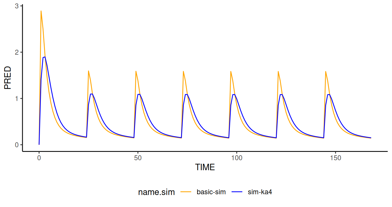
Example (modify): Change in formulation
This example edits the $PK section of an estimated
Nonmem model to adjust the model variable KA. Imagine we
are considering a new formulation, and we want to simulate how a
four-fold faster absorption would impact exposure. A simple way to do
that is to add a line KA=KA/4 to the $PK
section. Easy:
simres.ka4 <- NMsim(file.mod=file.mod,
                    data=data.sim,
                    name.sim="sim-ka4",
                    modify=list(PK=NMsim::add("KA=KA/4"))
                    )
simres.ka4 <- NMreadSim("simres-modify/xgxr021_simka4_MetaData.rds")Notice how the difference from the original simulation is that the
control stream has a new line in $PK reading exactly
KA=KA/4. This method works on the PK section alone and is
independent of what THETA and OMEGA parameters
are related to KA.
##      basic-sim$PK          | sim-ka4$PK
## [10] "V3=TVV3*EXP(ETA(4))" | "V3=TVV3*EXP(ETA(4))" [10]
## [11] "Q=TVQ*EXP(ETA(5))"   | "Q=TVQ*EXP(ETA(5))"   [11]
## [12] "S2=V2"               | "S2=V2"               [12]
##                            - "KA=KA/4"             [13]
The modify argument takes a list, where each element is
named as the control stream section to be modified, in this case
$PK. It can be - A character vector: the entire secion is
overwritten - A function: The function is applied to the section
text
In this case we used a function provided by NMsim called
add(). This function actually returns a function which is a
little complicated but serves the purpose of this example. The function
it returns appends KA=KA/4 to whatever character vector it
receives. It would be equivalent to do
simres.ka4 <- NMsim(file.mod=file.mod,
                    data=data.sim,
                    name.sim="sim-ka4",
                    ## equivalent to
                    ## modify=list(PK=NMsim::add("KA=KA/4"))
                    modify=list(PK=function(...)(c(...,"KA=KA/4")))
                    )
NMsim::add() may be a little easier to write and read.
It can also prepend text, see the pos argument. There is
also a function called NMsim::overwrite() which can replace
text strings. Once you try this one or two times, you will hopefully
appreciate how easily you can tweak control streams to do what you need,
still benifiting from NMsim()’s handling of data, automated
control stream generation etc.
Let’s compare the two simulation results. The absorption was slowed as expected.
Controlling Variables Using The Simulation Data Set
In the previous example KA was scaled by 4 by
specicification in the NMsim() call. The following example
uses a column in the simulation data set to scale the KA
value. This allows for a more flexible exploration of the effect of
different values of KA.
The effect on the concentration-time profile of a change in
formulation that reduces absorption rate KA is explored
with the use of a scaling factor KASCALE included to the
NONMEM control stream via the modify argument. The values
of KASCALE are provided through the NMsim
simulation data dat.sim.varka containing dosing events. We
simulate three distinct subjects, each with their own
KASCALE value. KASCALE values 1, 4, and 10 are
used, corresponding to an unchanged KA, a 4-fold, and a 10-fold larger
KA. We will be looking at PRED (of concentrations) so this
is effectively a typical subject analysis.
First KASCALE is added to the simulation data by
repeating the data set three for each value of KASCALE, and
redefining ID to be distinct for each value of
KASCALE. The code below uses data.table but
any data manipulation tool (such as base R or dplyr) could be used.
# add KASCALE and copy patient info for each value of KASCALE
dat.sim.varka <- data.sim[,data.table(KASCALE=c(1,4,10)),by=data.sim]
dat.sim.varka[,ID:=.GRP,by=.(KASCALE,ID)] # update patient IDs
setorder(dat.sim.varka,ID,TIME,EVID) # order rows
Then the NMsim() function is used to run the simulation
in which the modify argument is used to simulate a modified
model with different absorption rates, scaled by the parameter
KASCALE. Two different approaches are demonstrated:
- the effect of the scaling factor
KASCALEis added at the end of thePKsection in the NONMEM control stream.
simres.varka <- NMsim(file.mod=file.mod # NONMEM control stream
                     ,data=dat.sim.varka # simulation data file
                     ## ,name.sim="varka"
                     ,name.sim="add(): Append KA/KASCALE"
,modify=list(PK=add("KA=KA/KASCALE")))- the specific line that defines
TVKAis modified to include the effect of the scaling factorKASCALE. This is done for illustration ofoverwrite, see theinitsargument for how to edit parameter values directly.
simres.varka2 <- NMsim(file.mod=file.mod
                      ,data=dat.sim.varka
                       ##,name.sim="varka2"
                      ,name.sim="overwrite(): Replace THETA(1) by THETA(1)/KASCALE"
                      ,modify=list(PK=overwrite("THETA(1)","THETA(1)/KASCALE"))
                       )
The code below returns the plot
simres.both <- rbind(simres.varka,
                     simres.varka2)

ggplot(simres.both[EVID==2],aes(TIME,PRED,colour=factor(KASCALE)))+
    geom_line()+
    labs(colour="Fold absorption prolongation, KASCALE")+
    scale_x_continuous(breaks=seq(0,168,by=24))+
    facet_wrap(~name.sim)+
    scale_color_manual(values=c("orange", "blue", "darkgreen"))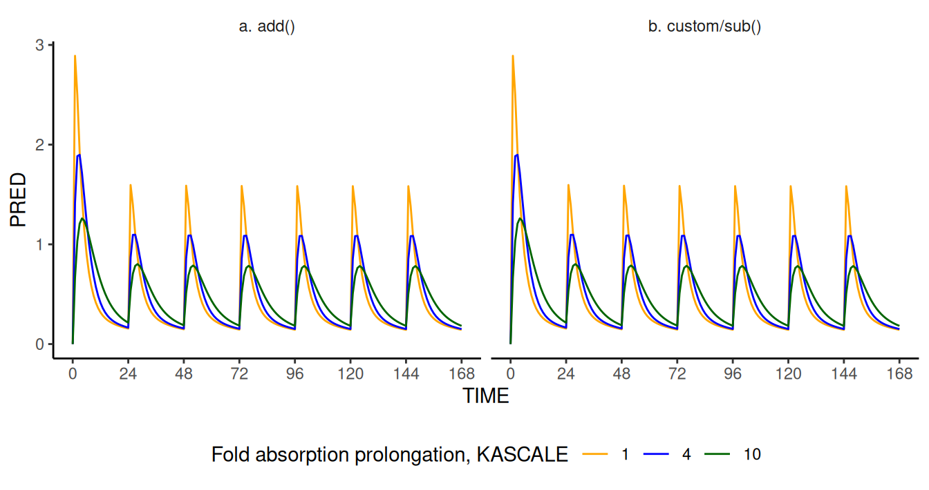
Concentration (PRED) profile as a function of time computed
by NMsim modified models a (left) and
b (right). The equivalence and robustness of the two
modified models is supported by the matching results, corresponding to
reduced PRED values for higher values of
KASCALE (lower absorption rate).
Additional modify Examples
modify example: Drug-Drug Interaction (DDI)
The effect of DDI on clearance (CL) and bioavailability
(F1) is simulated for the following scenarios
| scenario | CLSCALE | FSCALE | CLSCALE/FSCALE |
|---|---|---|---|
| noDDI | 1 | 1 | 1 |
| DDI.1 | 0.5 | 1.2 | 0.42 |
| DDI.2 | 0.33 | 1.1 | 0.3 |
First the CL and F1 data is added to the
patient data
## 'Outer join'
dat.sim.DDI=data.sim[,data.table(CLSCALE=c(1,1/2,1/3)
                                ,FSCALE=c(1,1.2,1.1)
                                ,lab=c("noDDI","DDI.1","DDI.2"))
                    ,by=data.sim]
dat.sim.DDI[,ID:=.GRP,by=.(lab,ID)]
setorder(dat.sim.DDI,ID,TIME,EVID)
Then, the DDI driven change in parameters is added at the end of the
PK section of the NONMEM control stream via the modify
argument in the NMsim() function.
simres.DDI <- NMsim(file.mod=file.mod
                   ,data=dat.sim.DDI
                   ,name.sim="DDI"
                   ,modify=list(PK=add("CL=CL*CLSCALE"
                                      ,"F1=FSCALE")))
The effect on the concentration-time profile is shown in the figure below
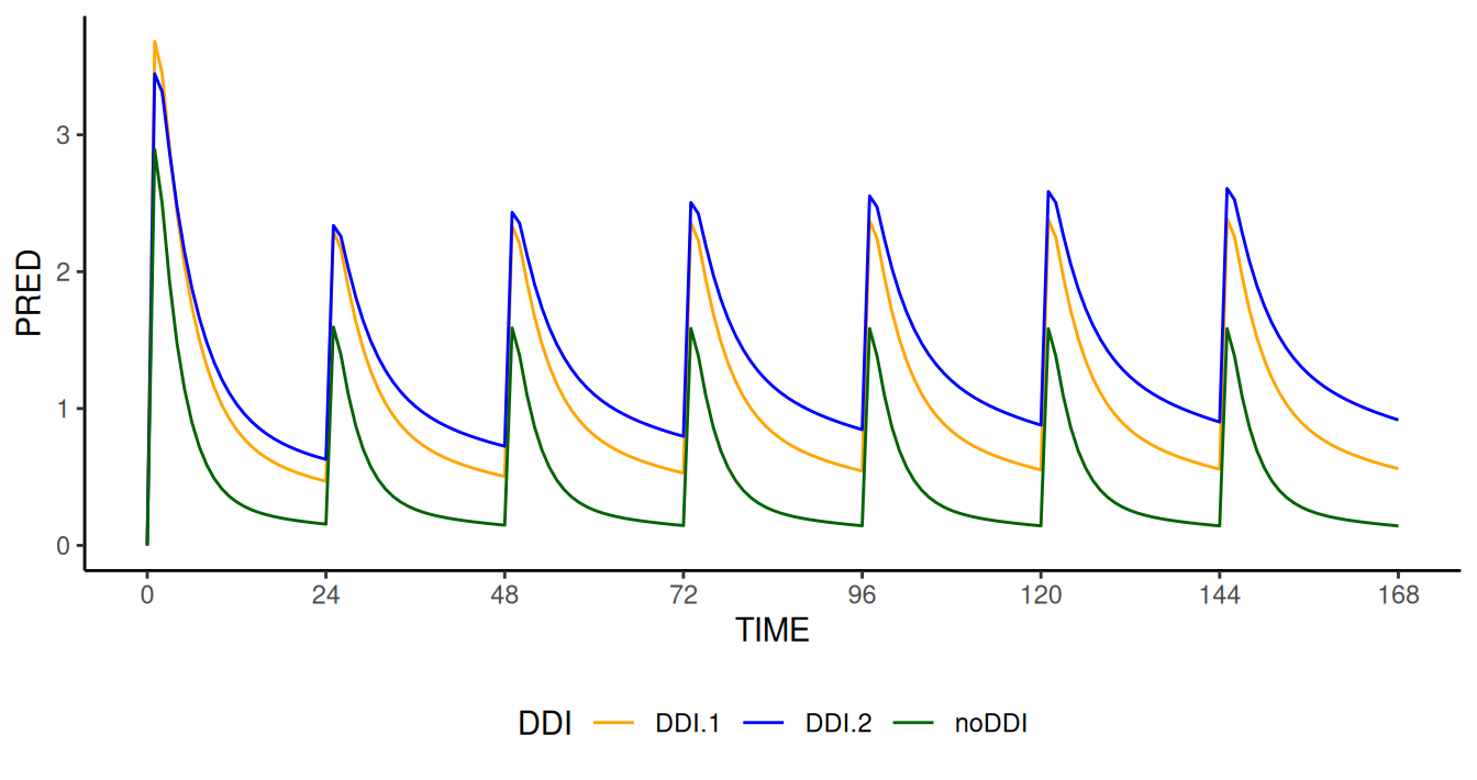
Concentration (PRED) profile as a function of time computed
by NMsim modified model for different DDIs. The modified
model correctly simulates (i) a higher value of Cmax on day
1 for higher biovalability; (ii) a higher PRED value at
steady state for lower apparent clearance effect
CLSCALE/FSCALE values.
modify example: Conditional Dose Delay
Deviations in the administration schedule of a drug are simulated
including three parameters in the dataset: the dose number
DOSCUMN, obtained with NMdata::addTAPD(), the
specific number of the delayed dose DELAYDOS and the time
delay ALAG.
dat.sim.alag = data.sim |> NMexpandDoses() |> addTAPD() # expand doses and add dose number
dat.sim.alag[,ROW:=.I] # restore ROW with correct value
                                        # add delayed dose
dat.sim.dos.delay=dat.sim.alag[,data.table(DELAYDOS=c(2,3,4,5,6,7))
                              ,by=dat.sim.alag]
                                        # add dose delay
dat.sim.alag.final=dat.sim.dos.delay[,data.table(ALAG=c(0,6,12,18,24))
                                    ,by=dat.sim.dos.delay]
                                        # update ID
dat.sim.alag.final[,ID:=.GRP,by=.(ALAG,DELAYDOS,ID)]
setorder(dat.sim.alag.final,ID,TIME,EVID)
                                        #dat.sim.alag.final = dat.sim.alag.final |> fill(DOSCUMN)
The following patient has a 6 hours delay to the administration of dose 2.
| TIME | AMT | DOSCUMN | DELAYDOS | ALAG |
|---|---|---|---|---|
| 0 | 300 | 1 | 2 | 6 |
| 24 | 150 | 2 | 2 | 6 |
| 48 | 150 | 3 | 2 | 6 |
| 72 | 150 | 4 | 2 | 6 |
| 96 | 150 | 5 | 2 | 6 |
| 120 | 150 | 6 | 2 | 6 |
| 144 | 150 | 7 | 2 | 6 |
The time delay is included in the modified control stream with
NMsim adding a single line at the end of the PK section,
where the dose delay on compartment 1 ALAG1 is modified for
the dose with dose number DOSCUMN equal to the target
delayed dose number DELAYDOS
simres.alag <- NMsim(file.mod=file.mod
                    ,data=dat.sim.alag.final
                    ,name.sim="alag"
                    ,modify=list(PK=
                                     add("IF(DOSCUMN.EQ.DELAYDOS) ALAG1=ALAG")))
The effect on concentration-time profiles and daily AUC are shown in the two images below.
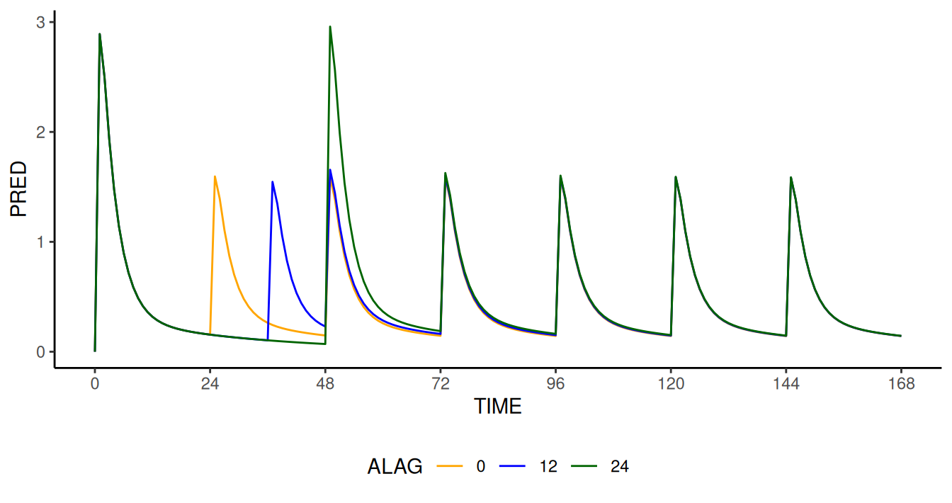
Effect of time delay (0, 12 and 24 hours on dose 2) on concentration
(PRED) profile as a function of time computed by
NMsim modified model. The implementation of the modified
model simply consists of the addition of the variables
DOSCUMN, DELAYDOS, and ALAG to
the original data set, and the addition of one line of code to the PK
section of the control stream via modify.
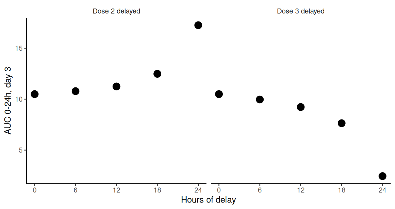
Daily exposure on day 3 as a function of time delay for dose 2 (left) and dose 3 (right). The simulation results predict an increased risk for possible safety concerns (left panel, over-exposure) and loss of efficacy (right panel, under-exposure) as dose time delay gets larger.
modify example: Calculation of AUC
The following example computes daily exposure:
- at post-processing, using trapezoidal method, after the unmodified
NONMEM model is simulated on three different fine grids with evenly
spaced time steps of
0.25,1, and4hours, respectively, labelled AUC trapez
file.mod.auc <- system.file("examples/nonmem/xgxr046.mod",
                            package="NMsim")
data.sim.auc <- NMreadCsv(system.file("examples/derived/dat_sim1.csv",
                                      package="NMsim"))
data.sim.auc[,AMT:=1000*AMT]

                                        # time step 1hr
data.sim.1hr=data.sim.auc
data.sim.1hr[,TSTEP:="1hr"]

                                        # time step 0.25hr
data.sim.0.25hr=addEVID2(data.sim.auc[EVID==1],CMT=2,time.sim=seq(0,192,by=0.25))
data.sim.0.25hr[,TSTEP:="0.25hr"]

                                        # time step 4hr
data.sim.4hr <- addEVID2(data.sim.auc[EVID==1],CMT=2,time.sim=seq(0,192,by=4))
data.sim.4hr[,TSTEP:="4hr"]

sres.trapez <- NMsim(file.mod=file.mod.auc
                    ,data=list(data.sim.1hr # run NMsim on a list of data sets to run all different scenarios at once
                              ,data.sim.0.25hr
                              ,data.sim.4hr)
                    ,seed=12345
                    ,table.vars=cc(PRED,IPRED)
                    ,name.sim="AUC.trapez"
                    ,reuse.results=reuse.results
                     )

                                        # daily AUC computation
sim.auc=sres.trapez[EVID==2,.(ID,TIME,PRED,time.step=TSTEP)]
sim.auc[,DAY:=(TIME%/%24)+1] # define DAY variable
                                        # create duplicate time steps for end-of-day
                                        # (e.g 24h belongs to both day 1 and day2)
sim.dupli.24h=sim.auc[TIME%%24==0 & TIME>0,.(ID
                                            ,DAY=DAY-1
                                            ,TIME
                                            ,PRED
                                            ,time.step)]
sim.auc.final <- rbind(sim.auc
                      ,sim.dupli.24h) |> setorder(ID,DAY,TIME,time.step)

sim.auc.trapez<-sim.auc.final[DAY<8,.(AUC=NMcalc::trapez(TIME,PRED))
                             ,by=.(ID,DAY,time.step)]
                                        # stmp=sres1[EVID==2,.(ID,TIME,PRED)]
                                        # stmp[,DAY:=(TIME%/%24)+1]
# sAUC<-stmp[,.(AUC=NMcalc::trapez(TIME,PRED)),by=.(ID,DAY)]- at run time, with an
NMsimmodified script, on a course grid with evenly spaced time steps of24hours, labelled AUC $DES. Of note, this task requires additions to the control stream in multiple sections.
# AUC with NMsim -  time step 24hr
data.sim2 <- addEVID2(data.sim.auc[EVID==1],CMT=2,time.sim=seq(0,by=24,length.out=9))

sres.des <- NMsim(file.mod=file.mod.auc
                 ,data=data.sim2
                 ,table.vars=cc(PRED,IPRED,AUCNMSIM)
                 ,name.sim="AUC.nmsim"
                 ,seed=12345
                 ,reuse.results=reuse.results
                 ,modify=list(MODEL=add("COMP=(AUC)")
                             ,DES=add("DADT(3)=A(2)/V2")
                             ,ERROR=add("AUCCUM=A(3)"
                                       ,"IF(NEWIND.NE.2) OLDAUCCUM=0"
                                       ,"AUCNMSIM = AUCCUM-OLDAUCCUM"
                                       ,"OLDAUCCUM = AUCCUM")))

sres.des[,DAY:=TIME%/%24]
sres.des[,AUC.NMsim:=AUCNMSIM]
sres.auc.des=sres.des[AUCNMSIM!=0,.(TIME,DAY,PRED,AUC.NMsim)]
The plot comparing the DES and trapez AUC
is obtained with the code below
sres.final=mergeCheck(sim.auc.trapez[,.(DAY,AUC,time.step)]
                     ,sres.auc.des[,.(DAY,AUC.NMsim)]
                     ,by="DAY")

ggplot(data=sres.final,aes(AUC.NMsim,AUC,colour=factor(time.step)))+
    geom_point(size=4)+
    labs(colour="Time step in fine grid")+
    scale_color_manual(values=c("orange", "blue", "darkgreen"))+
    xlim(c(0,17))+
    ylim(c(0,17))+
    ylab("AUC 0-24h by trapez method, on fine grid")+
    xlab("AUC 0-24h by integration through $DES, on coarse grid")+
    geom_abline(slope=1, intercept=0)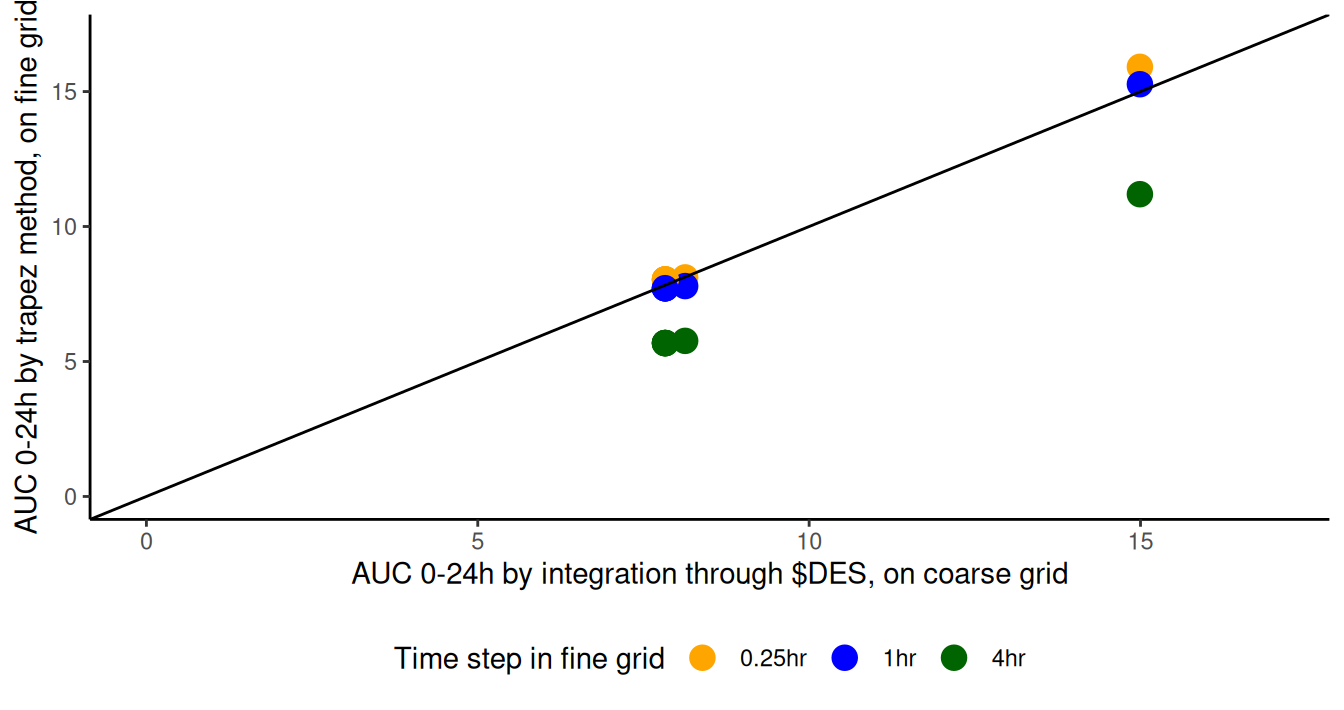
Daily exposures computed at run time ($DES, coarse grid, x-axis) and
post-processing time (trapez, fine grids, y-axis). AUC
(trapez) converges to the value computed with $DES method as the time
step is reduced. Includes identity line.
Modify $SIZES using sizes
For some NONMEM runs (simulations) it may be necessary to modify
$SIZES. Remember that the simulation control stream is
derived based on the estimation control stream, and so if
$SIZES settings are found in the estimation control stream,
those will by default also be in the simulation control stream generated
by NMsim(). The sizes argument is hence only
needed if the simulation $SIZES variables need to be
different from those used during estimation. This will typically be the
case due to properties of the simulation data. NMsim() by
default calls NONMEM with options that should help guessing some of
these options automatically, but here is how to do it if that fails.
sizes is very simple to use. As an example, this
NMsim() call sets $SIZES PD=100 LTV=70
sizes by default only overwrites matching
$SIZES variables. If $SIZES already contained
other variables than in this case PD and LTV,
those would be left untouched. If you want to write the
$SIZES section from scratch, add
wipe=TRUE:
Modify ACCEPT/IGNORE Using
filters
The filters argument is an interface to control the
ACCEPT and IGNORE (inclusion/exclusion)
statements in NONMEM. This can be but is rarely used for simulation
because the simulation data set is normally filtered for the simulation
purpose. The common exception is for simlation of VPC. To avoid
duplication of examples, please refer to