NMsim - Seamless NONMEM Simulation Platform in R

Philip Delff

November 18, 2024

Objectives

This introduction to NMsim aims at enabling NONMEM users to

• Configure NMsim to find your NONMEM installation
• Set up a simulation data set and simulate a NONMEM model using that data set
• Simulate a typical subject
• Simulate multiple models and compare them
• Simulate observed or previously simulated subjects based on emperical Bayes estimates (ETA’s)
• Simulate multiple subjects with covariate sampling and generation of prediction intervals

Configuration

NMsim must be configured with the path to the NONMEM executable. This can be done for each NMsim() call using the path.nonmem argument, but more easily it can be configured globally the following way. Also including where NMsim will run NONMEM and store intermediate files (dir.sims) and where to store final results (dir.res).

library(NMdata)
## Point NMsim to your NONMEM exectuable - looks like this on linux/osx
NMdataConf(path.nonmem = "/opt/NONMEM/nm75/run/nmfe75")
## or on Windows, it could be
NMdataConf(path.nonmem = "c:/nm75g64/run/nmfe75.bat")
NMdataConf(dir.sims="simtmp-intro", ## location of sim tmp files
           dir.res="simres-intro")  ## location of sim results

A first simulation with NMsim()

When providing a simulation data set, the default NMsim() behavior is to sample a new subject (ETA’s).

file.mod <- system.file("examples/nonmem/xgxr021.mod",
                        package="NMsim")
data.sim <- read.csv(system.file("examples/derived/dat_sim1.csv",
                                 package="NMsim"))
simres <- NMsim(file.mod=file.mod,data=data.sim)

Plot simulation results (click to show code)

datl <- as.data.table(simres) |>
    melt(measure.vars=cc(PRED,IPRED,Y))

plot1 <- ggplot(datl,aes(TIME,value,colour=variable))+
    geom_line(data=function(x)x[variable!="Y"])+
    geom_point(data=function(x)x[variable=="Y"])+
    labs(x="Hours since first dose",y="Concentration (ng/mL)",
         subtitle="Simulation of one new subject.",
         colour="")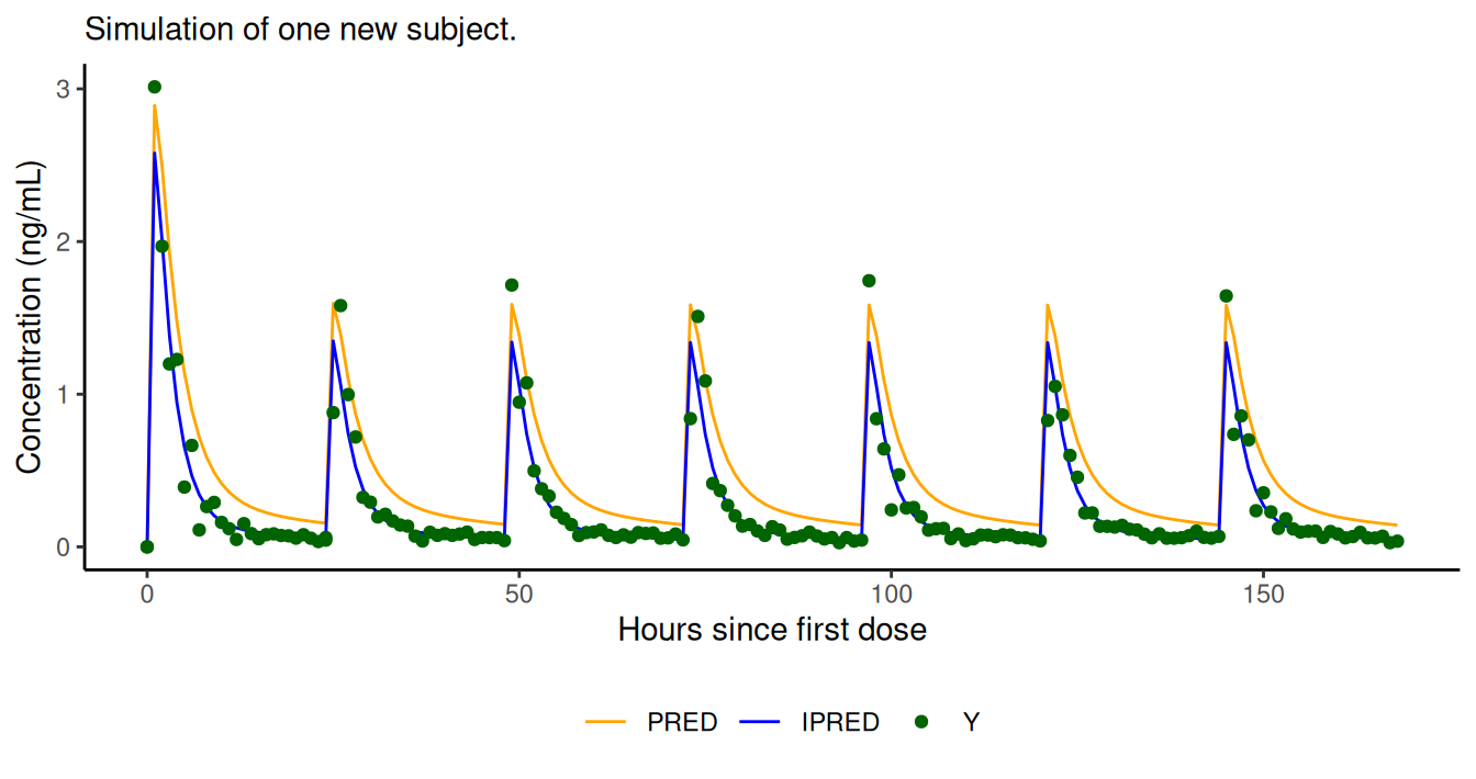
plot1

PRED, IPRED, and Y (if defined in control stream) are easily obtained with NMsim.

Notice that no information about the model is needed except for the control stream file path. The simulation is based on evaluation of PRED, IPRED, and optionally Y. Options exist for building more advanced simulation models. The models shown here are based on data available in the xgxr.

Simulation data sets

The simulation input data set is a data.frame, and NMsim() returns a data.frame.

The input data is a data.frame that

• Must contain at least the variables NONMEM will need to run the model (typically ID, CMT, AMT, etc. plus covariates)
• Can contain character variables (automatically carried to results)
• Column order does not matter

As long as those requirements are met, there are no requirements to how the data sets are created. So if you already have a prefered way to do this, that’s fine. NMsim provides convenient helper functions that can optionally be used. E.g., the data set used in these simulations can be created this way:

doses <- NMcreateDoses(TIME=c(0,24),AMT=c(300,150),
                       addl=list(ADDL=c(0,5),II=c(0,24)),CMT=1)
dat.sim <- addEVID2(doses,time.sim=0:(24*7),CMT=2)

Creating dosing regimens

NMcreateDoses() creates just the dosing events, and addEVID2() adds the sampling events. By default, doses are indicated using EVID=1 and samples by EVID=2.

Notice, NMcreateDoses() has convenient behaviours. See ?NMcreateDoses and the vignette ond creating simulation data sets for more.

Additional NMcreateDoses() examples

## arguments are expanded - makes loading easy
NMcreateDoses(TIME=c(0,12,24,36),AMT=c(2,1))

## Different doses by covariate
NMcreateDoses(TIME=c(0,12,24),AMT=data.table(AMT=c(2,1,4,2),DOSE=c(1,1,2,2))) 

Adding sampling times

For adding sampling times to a set of doses and/or samples, addEVID2() provides a similarly flexible interface. It accepts data.frames with covariates allowing for different sampling schemes for different subject groups (say different dosing regimens), and dosing times can be supplied relative to previous dosing times.

Additional addEVID2() examples

## a dosing data set with two doses
dt.dos <- NMcreateDoses(TIME=c(0,12),AMT=c(1))

## sampling based on time since previous dose
addEVID2(dt.dos,TAPD=1:2,CMT=2)

## TIME and TAPD can be combined - adding a follow-up
addEVID2(dt.dos,TAPD=1:2,TIME=96,CMT=2)

## sampling two compartments - naming them
addEVID2(dt.dos,TAPD=1:2,CMT=data.frame(CMT=2:3,DVID=c("Parent","Metabolite")))

Time since previous dose

While not used in these examples, it’s worth mentioning NMdata::addTAPD() for adding time since previous dose and other variables related to previous dose - previous dosing time, previous dose amount, cumulative number of doses, cumulative number of doses, and culative dose amount. These are often useful to add to a simulation dataset:

dat.sim <- addTAPD(dat.sim)

Check the simulation dataset

A quick way to check for a lot of common issues in a NONMEM data set is running NMcheckData():

NMcheckData(dat.sim,type.data="sim")

It is also advised to plot the simulation data set. See Creation of Simulation Data Sets for more details.

Typical subject simulation

• A typical subject is a subject with all ETAs = 0
• Covariates values are supplied using the simulation input data set
• typical=TRUE: replace all $OMEGA values with zeros

simres.typ <- NMsim(file.mod=file.mod,data=data.sim,
                    typical=TRUE,  ## FIX all OMEGA's to zero
                    name.sim="typical" ## simulation name - included in output
)

Simulate multiple models

Multiple models can be simulated using the same data set in one function call by supplying more than one model in the file.mod argument. The models can be simulated on multiple data sets by submitting a list of data.frames in the data argument. NMsim will return one data.frame with all the results for easy post-processing.

file2.mod <- "models/xgxr114.mod"
simres.typ2 <- NMsim(file.mod=c("2 compartments"=file.mod,
                                "1 compartment"=file2.mod),
                     data=data.sim,
                     typical=TRUE ## FIX all OMEGA's to zero
                     )
## The "model" column is used to distinguish the two models
subset(simres.typ2,EVID==2) |>
    ggplot(aes(TIME,PRED,colour=model))+
    geom_line()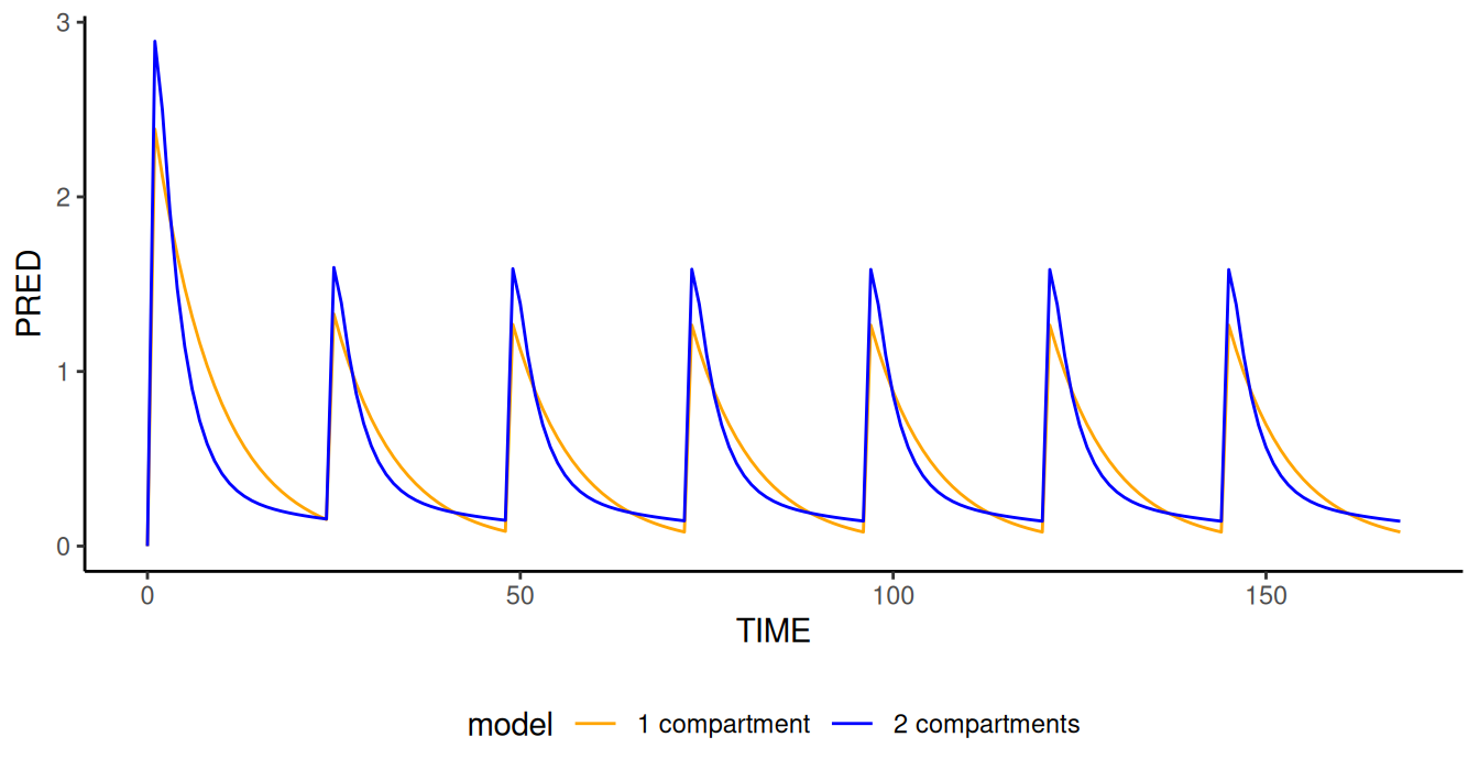

Simulation of multiple models and even multiple data sets is handled within one NMsim() call.

Emperical Bayes’ Estimates (known ETAs)

Reusing ETA’s is enabled using the NMsim_EBE method.

• By default, automatically re-uses estimated individual ETAs
• ID values in simulation data must match the ID values in the estimation that you want to simulate
• Other ETA sources (.phi files) can be specified
• Does not simulate residual variability - see addResVar() if needed
• Remember: Covariates may be needed in data set to fully reproduce the subjects’ parameters

In the following, we use table.vars to specify variables to output in NONMEM’s $TABLE section. In this case, we do that to make sure we get CL and V2. But generally, table.vars is very important to know as the very first thing to do to speed up NMsim(). This is because NONMEM often takes much longer writing the output table than it does doing the actual simulation. So it is recommended to specify a slim output table using something like table.vars=c("PRED","IPRED","Y") and other variables you may need from NONMEM. Notice NMsim knows how to combine output table data with the simulation input data, so you do not need variables like ID or TIME in table.vars.

## this example uses the same sim data for all subjects
res <- NMscanData(file.mod,quiet=T)
ids <- unique(res$ID)[1:5]
data.sim.ind <- merge(subset(data.sim,select=-ID),
                      data.frame(ID=ids))
setorder(data.sim.ind,ID,TIME,EVID)
simres.ebe <- NMsim(file.mod,
                    data=data.sim.ind,
                    method.sim=NMsim_EBE,
                    table.vars=c("CL","V2","IPRED","PRED")
)

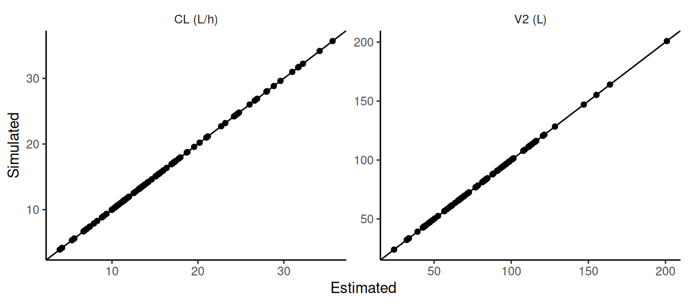
Individual parameters are confirmed to be identical in estimation results and simulation results

Prediction intervals

New subjects can be simulated in multiple ways with NMsim.

• If the input data set contains multiple subjects, these subjects will get separate random effects due to NONMEM $SIMULATION
• The subproblems argument translates to the SUBPROBLEMS NONMEM subroutine, replicating the simulation the specified number of times with new seeds
• The simPopEtas() function can generate a synthetic .phi file with a simulated population that can be reused in future NMsim() calls. This can be combined with simulation of covariates in R, allowing reuse of the same subjects across multiple simulations.

In the following we use both of these approaches to simulate 1000 new subjects. We use NMsim()’s name.sim argument to distinguish the simulation in output data and simulation output files.

Simulate 1000 new subjects using $SUBPROBLEMS

tablevars=cc(PRED,IPRED,Y)
simres.subprob <- NMsim(file.mod=file.mod,
                        data=data.sim,
                        name.sim="Subproblems", ## naming the simulation
                        subproblems=1000,  ## Will become SUPROBLEMS=1000 in NONMEM
                        table.vars=tablevars,
                        seed.R=764, ## NMsim() will set the R seed for reproducibility
                        reuse.results=reuse.results
                        )

Simulate 1000 new subjects with covariate sampling

## Replicating input data set allows for manual resampling of covariates.

## NMdata::findCovs() extracts unique values of column that do not vary within `by`. Since `by` is here the subject ID, that means we are finding subject level and globally equal variables only.
set.seed(2372)
Nsubjs <- 1000
dt.ids <- data.table(ID=1:Nsubjs)
dt.covs <- NMscanData(file.mod,quiet=T,as.fun="data.table") |>
    findCovs(by=c("ID"))
dt.ids[,IDEST:=sample(dt.covs[,ID],size=.N,replace=T)]
dt.ids <- mergeCheck(dt.ids,dt.covs[,.(IDEST=ID,WEIGHTB)],by="IDEST")

## This is data.table-style repeating `data.sim` without `ID` for each
## row in dt.ids. This is an outer join, or a cartesian product. I
## think in dplyr, one can use `crossing` to get this.
data.sim.nsubjs <- dt.ids[,subset(data.sim,select=-ID),by=dt.ids]
## see, we repeated one data set using the other
## dims(data.sim,dt.ids,data.sim.nsubjs)

## generate the population first, by simulating etas to use in the sim
simPopEtas(file.mod=file.mod,N=1000,seed=1231,
           file.phi="simres-intro/xgxr021_1000subjs.phi")
simres.datarep <- NMsim(file.mod=file.mod,
                        data=data.sim.nsubjs,
                        name.sim="Individual simulation data",
                        table.vars=tablevars,
                        seed.nm=103,
                        method.sim=NMsim_EBE,
                        file.phi="simres-intro/xgxr021_1000subjs.phi",
                        reuse.results=reuse.results
                        )

Derive and plot 90% prediction intervals

## Collect and stack simulation results 
simres.newpops <- rbind(as.data.table(simres.subprob),
                        simres.datarep,fill=T)[EVID==2]

## Derive prediction intervals - notice name.sim distincts results from the two methods
simres.pi <- simres.newpops[
   ,setNames(as.list(quantile(IPRED,probs=c(.05,.5,.95))),cc(ll,median,ul)),
    by=.(name.sim,trt,TIME)]

label.pi <- "90% Prediction interval"
simres.pi$type <- label.pi

p.pi <- ggplot(simres.pi,aes(TIME,fill=type))+
    geom_ribbon(aes(ymin=ll,ymax=ul),alpha=.4)+
    geom_line(aes(y=median,linetype="Median"))+
    scale_alpha_manual(values=setNames(c(.5),label.pi))+
    scale_linetype_manual(values=setNames(c(1),"Median"))+
    facet_wrap(~name.sim)+
    labs(x="Hours since first dose",y="Concentration (ng/mL)",colour="",linetype="")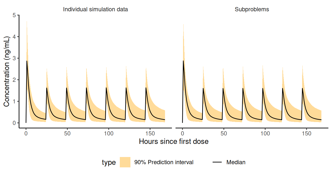

Prediction intervals. New subjects can be simulated in multiple ways with NMsim. A simulated population can be reused across simulations.

Read previously generated simulations

There is no need to save simulation results because they are already saved by NMsim. Instead, use arguments dir.sims, dir.res and name.sim to make sure to get a meaningful structure for the generated files. Then read the results with NMreadSim(). To re-read the first simulation we did in this article, we can do this:

simres <- NMreadSim("simres-intro/xgxr021_noname_MetaData.rds")

The folder and file names were constructed based on dir.res="simres-intro" and because name.sim was not provided for that first simulation, in which case “noname” is used as a placeholder. In fact, if we look at the console output from NMsim, it is telling us exactly that (look at the last line).

Click to show R console output from NMsim

> simres <- NMsim(file.mod=file.mod,data=data.sim)
Location(s) of intermediate files and Nonmem execution:
  simtmp-intro/xgxr021_noname
Location of final result files:
  simres-intro

* Writing simulation control stream(s) and simulation data set(s)
* Executing Nonmem job(s) 
Starting NMTRAN

(...)

Done with nonmem execution
* Collecting Nonmem results

Simulation results returned. Re-read them without re-simulating using:
  simres <- NMreadSim("simres-intro/xgxr021_noname_MetaData.rds")