Simulate Known Subjects Using Emperical Bayes Estimates (Etas/Phis)

Objectives

This vignettes aims at enabling you to use NMsim for the following purposes

Simualation of known subjects (estimated random effects),

Prerequisites

Simulation with known ETA values is only possible through NMsim’s internal Nonmem execution method. That means, we need to provide the path to the Nonmem executable.

NMdataConf(path.nonmem="/opt/NONMEM/nm75/run/nmfe75")

More information on configuration and test of configuration at NMsim-config.html.

You should be familiar with basic NMsim arguments as described in NMsim-intro.html. That vignette mostly talks about the default simulation method (new subjects). This vignette provides various examples on how the NMsim_EBE simulation method can be used to simulate “known” subjects. We shall explain in more detail what is meant by a “known subject”. Briefly it means their ETAs are known. The most common example of this is resimulation of subjects that were in the estimation data set.

Simulation of known subjects

We sometimes want to simulate the observed subjects, i.e. the subjects we included in the estimation data. We want to reuse the estimated random effects (ETA’s) given the subject ID’s. NMsim has a method for this called NMsim_EBE. The restriction is that all subjects (values of ID) in the simulation input data must have been used in the estimation input data.

For NMsim_EBE to work, ID values in the simulation data set must be identical to ID values used in the estimation. For models estimated with FOCEI, the ETAs are stored in the .phi file produced by Nonmem. This file must be available, and NMsim will automatically use it if applicable.

For EM-based estimation methods such as SAEM or IMP, NMsim cannot use the .phi file, and the user must have stored the ETAs in output table files for the method to work. It does not matter where in the table files they are, they just all need to be there. You can write all of them like it is done in the example model provided with NMsim called xgxr032.mod.

If using EM algorithms such as SAEM or IMP, remember to explicitly write ETAs to an output table in the Nonmem control stream:

$TABLE ETAS(1:LAST) NOAPPEND NOPRINT FILE=xgxr032_etas.txt

So a “subject” essentially means a set of ETAs. Covariates must still be provided in the input data set and can be modified if wanted. Notice, NMsim_EBE does nothing to restore covariates - you must define covariates in input data as needed.

Simulate known subjects on a new dosing regimen and new sample schedule

The following code takes an already created simulation data set with a single ID, and merges all other columns than ID onto the observed IDs. That gives the same simulation data for all subjects.

First thing, we decide on a model (an input control stream of an estimated model) to use for the example:

file.mod <- system.file("examples/nonmem/xgxr134.mod",package="NMsim")

We generate a simulation data set with a loading dose (300 mg) followed by 6 doses (150 mg) every 24 hours. For smoothness plotted curves we use hourly sampling.

doses <- NMcreateDoses(TIME=c(0,24),AMT=c(300,150),ADDL=5,II=24,CMT=1)
## Now we add the sample records using `NMaddSamples()`. 
dat.sim <- NMaddSamples(doses,TIME=0:(24*7),CMT=2)

## read model results just to extract the observed ID's. Notice, if
## your model uses covariates, those should be retrieved too.
res.mod <- NMscanData(file.mod,quiet=TRUE)
ids <- unique(res.mod[,c("ID","WEIGHTB","AGE","MALEN")])

## Repeat the simulation data set for each ID and order accordingly

## we will merge with all the observed subjects in stead of the single
## ID in the original data set.
dat.sim$ID <- NULL
dat.sim.known <- egdt(ids,
                      dat.sim
                      )
setorder(dat.sim.known,ID,TIME,EVID)
## check data
NMcheckData(dat.sim.known,type.data="sim")

simres.known <- NMsim(file.mod=file.mod,
                      data=dat.sim.known,
                      method.sim=NMsim_EBE,
                      table.vars="PRED IPRED CL V2 KA",
                      name.sim="known1"
                      )

And the simulation results are plotted for each subject.

ggplot(subset(simres.known,EVID==2),aes(TIME,IPRED,colour=factor(ID)))+
    geom_line()+
    theme(legend.position="none")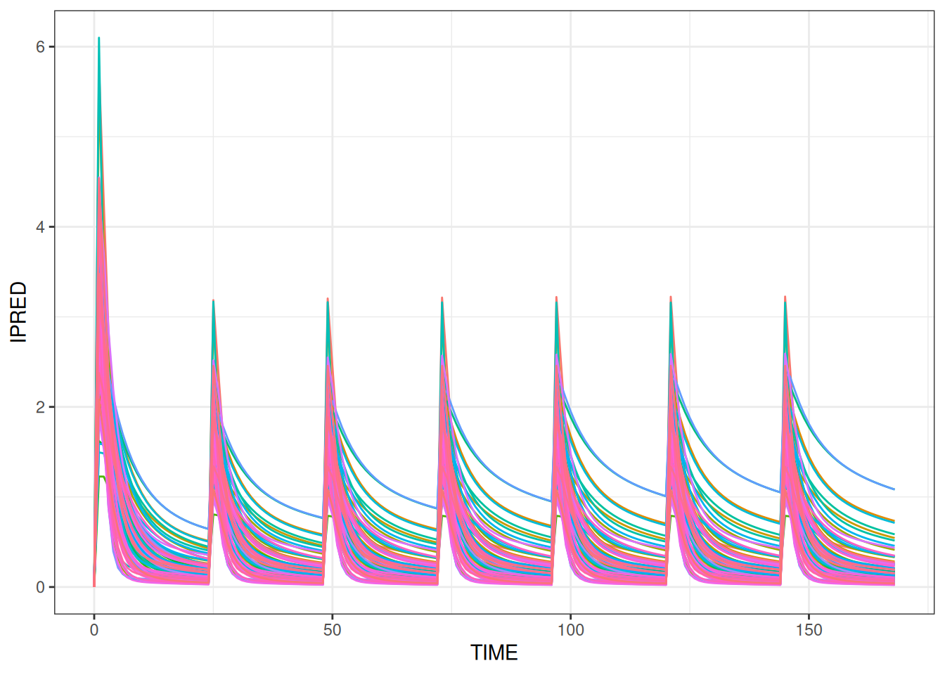

Individual dosing history, sample times or both

Individual simulations are useful for several purposes. Examples

Reuse individual dosing history and use a new common sample scheme. This could be for homogeneous evaluation of exposure metrics such as Cmax, AUC, or just to show concentration-time profiles at identical sampling times based on a model estimated on data with heterogeneos sampling. Currently, there is no example of this in this vignette but see the other examples, and it should be pretty clear how to do this.
Reuse dosing history and use individual sampling scheme from a different data set, e.g. PD.
Simulate a new common dosing and sampling scheme to simulate already observed subjects on a new regimen. This is sometimes done if for one reason or the other the model is not considered reliable for simulation of new subjects but the individual parameter estimates are trusted.
Reuse a simulated population. One may prefer to reuse the same simulated subjects in multiple simulations for reproducibility and to have all difference between say simulation results of different regimens be driven by differences in the regimen, and not in the populations. This use of NMsim_EBE is on the todo list tog get it’s own vignette here.

Simulate individual dosing history at new individual sampling times for a PK/PD dataset

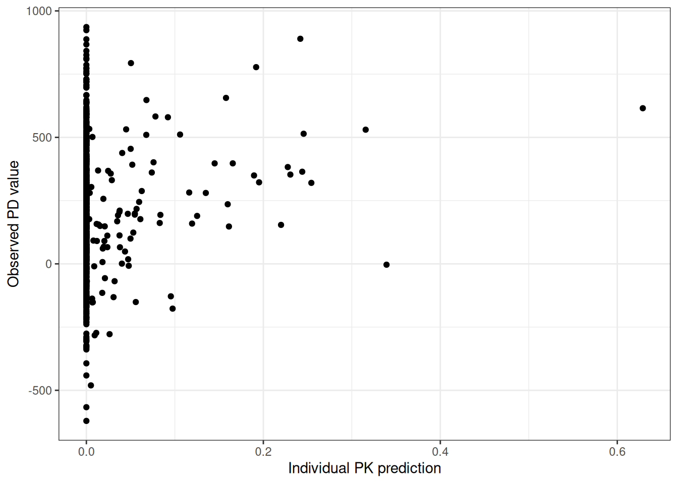
We want to plot some PD data angainst PK. However, PD was sampled differnetly than PK, and we want to evaluate the individual predictions of the PK model at the individual PD samplng times - reusing the individual dosing history.

Reading some example PD data:

pd <- readRDS(system.file("examples/data/xgxr_pd.rds",package="NMsim"))
## some code below makes use of data.table features so we make it a data.table
setDT(pd)

For a PK model without time-varying covariates, suggested steps to generate the data for the simulation are:

Take dose records from PK model estimation input data (pkdos). Just keep necessary columns like ID, TIME, EVID, CMT, AMT, ADDL, II, and any necessary covariates
Take PD data observation records (pdsamples). Just keep ID, TIME, and set EVID=2.
Add a unique row identifier to pdsamples (an integer row counter, like ROW=1:nrow(pdsamples))
Stack (rbind for data.tables or bind_rows in tidyverse) pkdos and pdsamples to one data set (pdsim)
In pdsim, set DV=NA
Sort pdsim at least by ID, TIME and EVID. There could be more depending on trial design

In case of time-varying covariates, you can keep all data records from the PK data (without DV), but change observation records to simulation records (EVID=2 instead of EVID=0).

## Take dose records from PK model estimation input data
pkres <- NMscanData(file.mod,quiet=TRUE)
pkdos <- pkres[EVID==1,.(ID, TIME, EVID, CMT, AMT)]
## Take PD data observation records (`pdsamples`)
pdsamples <- pd[EVID==0,.(ID,TIME,LIDV)]
## Stack `pkdos` and `pdsamples` to one data set (`pdsim`)
pdsim <- rbind(pkdos,pdsamples,fill=TRUE)
## Nonmem needs a DV column to run
pdsim[,DV:=NA]
## only include subjects that were included in the PK model
pdsim <- pdsim[ID%in%pkres$ID]
setorder(pdsim,ID,TIME,EVID)

Then run NMsim like this. We are renaming the prediction columns using Nonmem $TABLE statement not to confuse PK predictions and PD predictions.

simres.pksim <- NMsim(file.mod,
                      data=pdsim,
                      name.sim="pkpd",
                      method.sim=NMsim_EBE,
                      table.vars="PKIPRED=IPRED PKPRED=PRED"
                      )

ggplot(simres.pksim[!is.na(LIDV)&!is.na(PKIPRED)],aes(PKIPRED,LIDV))+
    geom_point()+
    labs(x="Individual PK prediction",y="Observed PD value")