Data Set Creation with NMsim
Philip Delff
July 21, 2026 using NMsim 0.2.7.901
Source:vignettes/NMsim-DataCreate.Rmd
NMsim-DataCreate.RmdIntroduction
The purpose of data sets of interest in this vignette is succesfull
and meaningful simulation with NMsim().
The data argument to NMsim() is essential to any simulation. For a
simulation of new subjects, the data may be the only need
argument In addition to a control stream file path.
simres <- NMsim(file.mod=file.mod,data=data.sim)NMsim and NMdata provide concise and
feature-rich methods to create and check such data sets.
NMsim() does not require simulation data sets to be created using
NMsim functions. If already accustumed to other data set generation
tools, you can most likely continue using those with
NMsim().
However created, The NMsim() data argument must
- be a
data.frame - its columns names are exact NONMEM
$DATAvariables
Checking the data set before running Nonmem can significantly
simplify identification of data set issues. This vignette uses
NMdata::NMcheckData for automated checks of several value
types and other properties of data sets. Like NMsim,
NMdata::NMcheckData does not depend on how the data set was
created.
Create Dosing Events
NMcreateDoses() is a flexible function that creates
dosing records based on a concise syntax. As an example we create a
regimen with a loading dose of 300 mg followed by 150 QD for 6 days (7
doses in total). We dose into compartment 1, and we want to simulate
samples in the second compartment. These numbers depend on the model
which the data set is intended to be used with.
doses <- NMcreateDoses(TIME=seq(0,by=24,length.out=7),
                       AMT=c(300,150),CMT=1)
doses| ID | TIME | EVID | CMT | AMT | MDV |
|---|---|---|---|---|---|
| 1 | 0 | 1 | 1 | 300 | 1 |
| 1 | 24 | 1 | 1 | 150 | 1 |
| 1 | 48 | 1 | 1 | 150 | 1 |
| 1 | 72 | 1 | 1 | 150 | 1 |
| 1 | 96 | 1 | 1 | 150 | 1 |
| 1 | 120 | 1 | 1 | 150 | 1 |
| 1 | 144 | 1 | 1 | 150 | 1 |
Since the most common dosing regimens consists of a potential loading
dose or a series of loading doses, followed by a maintenance regimen,
NMcreateDoses() is designed to expand variables to match
the the lenght of TIME, by repeating the last
value. Notice above, how AMT=300 is not repeated -
only AMT=150 is. This is a NMcreateDoses()
feature and is different from how say data.frame() would
cycle variables to match the lengths.
We can also use ADDL/II to get an equivalent result.
### multiple dose regimens with loading are easily created with NMcreateDoses too
## We use ADDL+II (either method easy)
doses <- NMcreateDoses(TIME=c(0,24),AMT=c(300,150),ADDL=5,II=24,CMT=1)
## doses$trt <- "300 mg then 150 mg QD"
## Notice, the ID and MDV columns are included
doses| ID | TIME | EVID | CMT | AMT | II | ADDL | MDV |
|---|---|---|---|---|---|---|---|
| 1 | 0 | 1 | 1 | 300 | NA | NA | 1 |
| 1 | 24 | 1 | 1 | 150 | 24 | 5 | 1 |
Notice how ADDL and II are by default only
applied to the last dosing event (this behavior is controlled by the
addl.lastonly argument).
doses2 <- NMcreateDoses(TIME=seq(0,by=24,length.out=7),
                        AMT=c(300,150),CMT=1)
## doses2$trt <- "300 mg then 150 mg QD"
doses2| ID | TIME | EVID | CMT | AMT | MDV |
|---|---|---|---|---|---|
| 1 | 0 | 1 | 1 | 300 | 1 |
| 1 | 24 | 1 | 1 | 150 | 1 |
| 1 | 48 | 1 | 1 | 150 | 1 |
| 1 | 72 | 1 | 1 | 150 | 1 |
| 1 | 96 | 1 | 1 | 150 | 1 |
| 1 | 120 | 1 | 1 | 150 | 1 |
| 1 | 144 | 1 | 1 | 150 | 1 |
The difference between doses and doses2 is
that doses2 is “expanded” with separate dosing event rows
for each dose. In some cases, the expanded format is more convenient.
NMdata::NMexpandDoses() expands the ADDL and
II:
NMexpandDoses(doses)| ID | TIME | EVID | CMT | AMT | II | ADDL | MDV |
|---|---|---|---|---|---|---|---|
| 1 | 0 | 1 | 1 | 300 | NA | NA | 1 |
| 1 | 24 | 1 | 1 | 150 | 0 | 0 | 1 |
| 1 | 48 | 1 | 1 | 150 | 0 | 0 | 1 |
| 1 | 72 | 1 | 1 | 150 | 0 | 0 | 1 |
| 1 | 96 | 1 | 1 | 150 | 0 | 0 | 1 |
| 1 | 120 | 1 | 1 | 150 | 0 | 0 | 1 |
| 1 | 144 | 1 | 1 | 150 | 0 | 0 | 1 |
Additional NMcreateDoses() examples
Arguments Lengths are Expanded to Match Time
Arguments are expanded to match length of TIME - makes
loading easy.
NMcreateDoses(TIME=c(0,12,24,36),AMT=c(2,1))| ID | TIME | EVID | CMT | AMT | MDV |
|---|---|---|---|---|---|
| 1 | 0 | 1 | 1 | 2 | 1 |
| 1 | 12 | 1 | 1 | 1 | 1 |
| 1 | 24 | 1 | 1 | 1 | 1 |
| 1 | 36 | 1 | 1 | 1 | 1 |
Covariates can be provided by making variables a
data.frame with the variable and a covariate. Here,
AMT is different for two subjects with DOSE=1
and DOSE=2, respectively. This means for each of the
subjects, AMT is of length two, hence they are expanded to
match the length (3) of TIME.
NMcreateDoses(TIME=c(0,12,24),AMT=data.table(AMT=c(2,1,4,2),DOSE=c(1,1,2,2))) | ID | TIME | EVID | CMT | AMT | MDV | DOSE |
|---|---|---|---|---|---|---|
| 1 | 0 | 1 | 1 | 2 | 1 | 1 |
| 1 | 12 | 1 | 1 | 1 | 1 | 1 |
| 1 | 24 | 1 | 1 | 1 | 1 | 1 |
| 2 | 0 | 1 | 1 | 4 | 1 | 2 |
| 2 | 12 | 1 | 1 | 2 | 1 | 2 |
| 2 | 24 | 1 | 1 | 2 | 1 | 2 |
Multiple Endpoints (e.g. parent and metabolite)
Pass a data.frame to NMaddSamples()’s CMT
argument to include multiple endpoints.
NMaddSamples(doses,CMT=data.frame(CMT=c(2,3),DVID=c("Parent","Metabolite")),TIME=1:2)| ID | TIME | EVID | CMT | AMT | II | ADDL | MDV | DVID |
|---|---|---|---|---|---|---|---|---|
| 1 | 0 | 1 | 1 | 300 | NA | NA | 1 | NA |
| 1 | 1 | 2 | 2 | NA | NA | NA | 1 | Parent |
| 1 | 1 | 2 | 3 | NA | NA | NA | 1 | Metabolite |
| 1 | 2 | 2 | 2 | NA | NA | NA | 1 | Parent |
| 1 | 2 | 2 | 3 | NA | NA | NA | 1 | Metabolite |
| 1 | 24 | 1 | 1 | 150 | 24 | 5 | 1 | NA |
Cohort-Dependent or Individual Sampling Schemes
Same way as for the CMT argument, TIME can
also be a data.frame. If it contains a covariate found in
the doses data, the added simulation times will be merged on
accordingly. You can use say a cohort identifier, or it could be
ID which allows you to reuse (all or parts of) the observed
sample times.
Add Sampling Events
Now we add the sample records using NMaddSamples().
## Add simulation records - longer for QD regimens
dat.sim <- NMaddSamples(doses,TIME=0:(24*7),CMT=2)
Additional NMaddSamples() examples
These examples serve to show the behavior of
NMaddSamples(), specifically. Hence, a simple dosing data
set with just two doses is used.
dt.dos <- NMcreateDoses(TIME=c(0,12),AMT=c(1))Sampling based on time since previous dose:
NMaddSamples(dt.dos,TAPD=1:2,CMT=2)| ID | TIME | EVID | CMT | AMT | MDV | TAPD |
|---|---|---|---|---|---|---|
| 1 | 0 | 1 | 1 | 1 | 1 | NA |
| 1 | 1 | 2 | 2 | NA | 1 | 1 |
| 1 | 2 | 2 | 2 | NA | 1 | 2 |
| 1 | 12 | 1 | 1 | 1 | 1 | NA |
| 1 | 13 | 2 | 2 | NA | 1 | 1 |
| 1 | 14 | 2 | 2 | NA | 1 | 2 |
TIME and TAPD can be combined - adding a
follow-up
NMaddSamples(dt.dos,TAPD=1:2,TIME=96,CMT=2)| ID | TIME | EVID | CMT | AMT | MDV | TAPD |
|---|---|---|---|---|---|---|
| 1 | 0 | 1 | 1 | 1 | 1 | NA |
| 1 | 1 | 2 | 2 | NA | 1 | 1 |
| 1 | 2 | 2 | 2 | NA | 1 | 2 |
| 1 | 12 | 1 | 1 | 1 | 1 | NA |
| 1 | 13 | 2 | 2 | NA | 1 | 1 |
| 1 | 14 | 2 | 2 | NA | 1 | 2 |
| 1 | 96 | 2 | 2 | NA | 1 | NA |
## sampling two compartments - naming them
NMaddSamples(dt.dos,TAPD=1:2,CMT=data.frame(CMT=2:3,DVID=c("Parent","Metabolite")))| ID | TIME | EVID | CMT | AMT | MDV | TAPD | DVID |
|---|---|---|---|---|---|---|---|
| 1 | 0 | 1 | 1 | 1 | 1 | NA | NA |
| 1 | 1 | 2 | 2 | NA | 1 | 1 | Parent |
| 1 | 1 | 2 | 3 | NA | 1 | 1 | Metabolite |
| 1 | 2 | 2 | 2 | NA | 1 | 2 | Parent |
| 1 | 2 | 2 | 3 | NA | 1 | 2 | Metabolite |
| 1 | 12 | 1 | 1 | 1 | 1 | NA | NA |
| 1 | 13 | 2 | 2 | NA | 1 | 1 | Parent |
| 1 | 13 | 2 | 3 | NA | 1 | 1 | Metabolite |
| 1 | 14 | 2 | 2 | NA | 1 | 2 | Parent |
| 1 | 14 | 2 | 3 | NA | 1 | 2 | Metabolite |
Use the by argument to specify separate sampling times
for different subsets of subjects.
dt.dos2 <- NMcreateDoses(TIME=c(0,12,24),AMT=data.table(AMT=c(2,1,4,2),DOSE=c(1,1,2,2)))
NMaddSamples(dt.dos2,TIME=data.frame(TIME=c(1:2,1:4),DOSE=c(rep(1,2),rep(2,4))),CMT=2,by="DOSE")| ID | TIME | EVID | CMT | AMT | MDV | DOSE |
|---|---|---|---|---|---|---|
| 1 | 0 | 1 | 1 | 2 | 1 | 1 |
| 1 | 1 | 2 | 2 | NA | 1 | 1 |
| 1 | 2 | 2 | 2 | NA | 1 | 1 |
| 1 | 12 | 1 | 1 | 1 | 1 | 1 |
| 1 | 24 | 1 | 1 | 1 | 1 | 1 |
| 2 | 0 | 1 | 1 | 4 | 1 | 2 |
| 2 | 1 | 2 | 2 | NA | 1 | 2 |
| 2 | 2 | 2 | 2 | NA | 1 | 2 |
| 2 | 3 | 2 | 2 | NA | 1 | 2 |
| 2 | 4 | 2 | 2 | NA | 1 | 2 |
| 2 | 12 | 1 | 1 | 2 | 1 | 2 |
| 2 | 24 | 1 | 1 | 2 | 1 | 2 |
The doses can be replicated to multiple ID’s using the N
argument. Default is N=1. If N=1 results in
two distinct subjects, N=100 will result i 200 distinct
subjects. The ID column will automatically be recoded to contain
distinct ID’s.
Adding Time After Previous Dose and Related Information
While not necessary for NMsim() to run, it’s worth
mentioning NMdata::addTAPD() for adding time since previous
dose and other variables related to previous dose - previous dosing
time, previous dose amount, cumulative number of doses, cumulative
number of doses, and culative dose amount. These are often useful to add
to a simulation dataset, especially for postprocessing:
| ID | TIME | EVID | CMT | AMT | II | ADDL | MDV | DOSCUMN | TPDOS | TAPD | PDOSAMT | DOSCUMA |
|---|---|---|---|---|---|---|---|---|---|---|---|---|
| 1 | 0 | 1 | 1 | 300 | NA | NA | 1 | 1 | 0 | 0 | 300 | 300 |
| 1 | 0 | 2 | 2 | NA | NA | NA | 1 | 0 | NA | NA | NA | 0 |
| 1 | 1 | 2 | 2 | NA | NA | NA | 1 | 1 | 0 | 1 | 300 | 300 |
| 1 | 2 | 2 | 2 | NA | NA | NA | 1 | 1 | 0 | 2 | 300 | 300 |
| 1 | 3 | 2 | 2 | NA | NA | NA | 1 | 1 | 0 | 3 | 300 | 300 |
| 1 | 4 | 2 | 2 | NA | NA | NA | 1 | 1 | 0 | 4 | 300 | 300 |
Notice TAPD for the sample at TIME==0.
addTAPD() does not use the order of the data set to
determine the time-order or the records. The default behavior of
addTAPD is to treat a sample taken at the exact same time
as a dose as a pre-dose. If instead we want them to be considered
post-dose, we have to specify how to order EVID
numbers.
## order.evid=c(1,2) means doses are ordered before EVID=2 records
dat.sim2 <- addTAPD(dat.sim,order.evid=c(1,2))
## now the TIME=0 sample has TAPD=0
head(dat.sim2)| ID | TIME | EVID | CMT | AMT | II | ADDL | MDV | DOSCUMN | TPDOS | TAPD | PDOSAMT | DOSCUMA |
|---|---|---|---|---|---|---|---|---|---|---|---|---|
| 1 | 0 | 1 | 1 | 300 | NA | NA | 1 | 1 | 0 | 0 | 300 | 300 |
| 1 | 0 | 2 | 2 | NA | NA | NA | 1 | 1 | 0 | 0 | 300 | 300 |
| 1 | 1 | 2 | 2 | NA | NA | NA | 1 | 1 | 0 | 1 | 300 | 300 |
| 1 | 2 | 2 | 2 | NA | NA | NA | 1 | 1 | 0 | 2 | 300 | 300 |
| 1 | 3 | 2 | 2 | NA | NA | NA | 1 | 1 | 0 | 3 | 300 | 300 |
| 1 | 4 | 2 | 2 | NA | NA | NA | 1 | 1 | 0 | 4 | 300 | 300 |
addTAPD() uses NMdata::NMexpandDoses() to
make sure all dosing times are considered. See
?NMdata::addTAPD for what the other created columns mean
and for many useful features.
Finalizing and Checking the Simulation Data
dat.sim is now a valid simulation data set with one
subject. However, even though NMaddSamples() does try to
order the data in a meaningful way, it is recommended to always manually
order the data set. We use data.table’s
setorder(). base::order or
dplyr::arrange can just as well be used. A row identifier
(counter) is not needed for NMsim but it can make post-processing
easier, so we add that too.
NMsim does not include plotting functionality, but here
is a simple way to show dosing amounts and sample times.
NMdata::NMexpandDoses() is used to expand the
doses coded with ADDL/II in order to get a
data row to plot for each dose. We also take the sum of the amounts by
time point in case doses are simultaneous.
dtplot <- NMdata::NMexpandDoses(dat.sim,as.fun="data.table")
dtplot <- dtplot[,.(AMT=sum(AMT)),by=.(ID,CMT,TIME,EVID)]

ggplot(dtplot,aes(TIME,factor(CMT),colour=factor(EVID)))+
    geom_point(data=function(x)x[EVID==1],aes(size=AMT))+
    geom_point(data=function(x)x[EVID==2],shape="|")+
    labs(x="Time (hours)",y="Compartment",shape="EVID",colour="EVID")+
    theme(legend.position="bottom")
#> Ignoring unknown labels:
#> • shape : "EVID"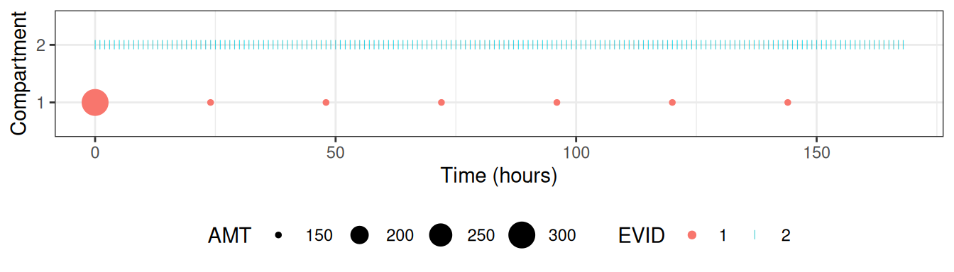
After using NMexpandDoses() the simulation data set is
plotted.
A brief overview of the number of events broken down by event type
EVID and dose amount AMT:
NMexpandDoses(dat.sim)[,.(Nrows=.N),keyby=.(CMT,EVID,AMT)] | CMT | EVID | AMT | Nrows |
|---|---|---|---|
| 1 | 1 | 150 | 6 |
| 1 | 1 | 300 | 1 |
| 2 | 2 | NA | 169 |
Showing the top five rows for understanding what the data now looks like. Notice that the following are not issues:
- Data contains a mix of numeric and non-numeric columns
- Columns are not sorted in Nonmem-friendly style with non-numeric columns to the right
| ID | TIME | EVID | CMT | AMT | II | ADDL | MDV | ROW |
|---|---|---|---|---|---|---|---|---|
| 1 | 0 | 1 | 1 | 300 | NA | NA | 1 | 1 |
| 1 | 0 | 2 | 2 | NA | NA | NA | 1 | 2 |
| 1 | 1 | 2 | 2 | NA | NA | NA | 1 | 3 |
| 1 | 2 | 2 | 2 | NA | NA | NA | 1 | 4 |
| 1 | 3 | 2 | 2 | NA | NA | NA | 1 | 5 |
Finally, We check the simulation data set for various potential
issues in Nonmem data sets using NMdata::NMcheckData and
summarize the number of doses and observations:
NMdata::NMcheckData(dat.sim,type.data="sim")
#> No findings. Great!
As already mentioned, column order does not matter to NMsim.
But Be aware that NMsim() does not reorder rows
before simulation. The user is responsible for ordering the rows of the
simulation data.
Other features
The default behavior of NMaddSamples() is to use
EVID=2 (which means they are neither doses, samples, nor
resetting events) for the added records. Should you want to change that
(maybe to EVID=0), use the EVID argument.