Simulation-Based Forest Plots with NMsim

NMsim

Introduction

The forest plot is an effective and widely recognized way to illustrate estimated covariate effects on exposure or response, or parameters related to these (e.g. clearance). The forest plot typically includes precision of the estimate in terms of a confidence interval. NMsim provides highly automated methods for simulation of Nonmem models for generation of forest plots.

Objectives

This short demonstration of generation of simulation-based forest plots using NMsim is intended to make the user ready to perform the following steps.

Generate simulation data sets designed for forest plot simulations
- Dosing and sampling scheme using NMcreateDoses()
- Define covariates to simulate using forestDefineCovs()
Simulate with parameter uncertainty by one of
- Based on $COV using NMsim_NWPRI()
- Based on $COV using NMsim_VarCov()
- Using an existent bootstrap estimation (e.g. from PSN)
Postprocess simulation for plotting/tabulation
- Define end-points, such as an AUC, Cmax or any simulation-based endpoint
- Summarize covariate effect estimates with confidence intervals, using forestSummarize()
Plot the summary as a forest plot

Each step is facilitated with efficient interfaces (R functions) and automated execution. Essentially, each step above is one function call. The results from all methods are compared in one plot.

Plotting is includied in the example using the coveffectsplot package. Other packages or user’s own scripts can be used for plotting.

We shall focus the main example to be simple and general. Hopefully, the user will be able to customize and apply a similar workflow to their own models with minimum effort. Folded code-chunks and references will be provided for additional features.

Prerequisites

An estimated Nonmem model - at least, input control stream and .ext file.
- If simulating based on $COVARIANCE, the .cov file.
- If simulating based on bootstrap, either a summary of or all the .ext files from the boot strap estimations must be available.
- If references and/or covariate quantile values are to be calculated by NMsim (easiest option), ideally all output ($TABLE) data sets and the input data set used for the estimation are available.
Familiarity with NMsim-intro.html, at least including “A first simulation with NMsim()”.
Configuration of NMsim so user can succesfully do simulation using NMsim().
Familiarity with methods to simulate with parameter uncertainty can be helpful. Before settling on your final forest plot simulation, it is recommended to understand pros and cons of the different methods provided by NMsim as described in NMsim-ParamUncertain.html.

Background

Forest plots include a confidence interval of the estimated or simulated effect. The confidence interval is derived from uncertainy estimates of the parameter set. This is not between-subject variability (BSV), also called intra-individual variability. For NMsim to simulate the distribution of the covariate effect, this uncertainty must be obtained through one of two sources. Either as the result of a succesfull $COVARIANCE step on the model, or using an already executed bootstrap.

In some cases, the forest plot can be derived based on model estimates without simulation. This is the case for a forest plots of PK parameters such as clearance when a covariance step is available, and it can be the case with forest plots of exposure metrics if the PK is linear and only steady-state average concentration (or AUC) is of interest. If the PK is non-linear and/or exposure metrics such as Cmax which depends on multiple PK parameters are of interest, a simulation-based forest plot may be needed. As we shall see, NMsim provides a flexible and concise framework to perform the required. In fact, the simulation-based workflow is so general and easy to perform that it may be prefered even in cases where simulation is not needed.

Initialization

library(data.table)
library(NMsim)
library(NMdata)  
library(NMcalc)  ## Optional. Used to calculate AUC.
library(coveffectsplot) ## used for plotting
library(knitr) ## for printing tables with knitr::kable
library(ggplot2)
library(ggstance)

theme_set(theme_bw())

NMdataConf(
    path.nonmem = "/opt/NONMEM/nm75/run/nmfe75", ## path to NONMEM executable
    dir.sims="simtmp-forest", ## where to store temporary simulation results
    dir.res="simres-forest"   ## where to store final simulation results
)

A model is selected.

## file.mod <- "NMsim-forest-models/xgxr134.mod"
file.mod <- system.file("examples/nonmem/xgxr134.mod",package="NMsim")

Generation of simulation input data

Dosing and sampling

The simulation data set has to match the model in compartment numbers, and it must contain all variables needed to run the NONMEM model. We simulate daily dosing of 30 mg. col.id=NA to omit a subject id in doses as we will instead reuse it for multiple subjects.

doses <- NMcreateDoses(TIME=0,AMT=30,ADDL=30,II=24)
doses

ID	TIME	EVID	CMT	AMT	II	ADDL	MDV
1	0	1	1	30	24	30	1

We sample every 15 minutes on the first day and one day in steady-state.

## add a sampling scheme
time.sim <- c(
    seq(0,24,.25), ## Day 1
    seq(0,24,.25)+30*24 ## Steady-State
)
dt.sim <- addEVID2(doses,TIME=time.sim,CMT=2,as.fun="data.table")

## `addEVID2()` has been renamed to `NMaddSamples()`. `addEVID2()` still works to ensure
## backward-compatibility.

dt.sim[TIME<=24,period:="Day 1"]
dt.sim[TIME>=30*24&TIME<=31*24,period:="Steady-State"]

The following table summarizes the number of doses and samples. Notice, the doses are repeated.

period	EVID	ADDL	II	N
Day 1	1	30	24	1
Day 1	2	NA	NA	97
Steady-State	2	NA	NA	97

How to sample multiple endpoints

There is only one analyte in this data set. If for instance, you have a parent and a metabolite, adding sampling times could look like this:

dt.sim.parent.metab <-
    addEVID2(doses,TIME=time.sim,CMT=data.frame(analyte=c("parent","metabolite"),CMT=c(2,3)))

## `addEVID2()` has been renamed to `NMaddSamples()`. `addEVID2()` still works to ensure
## backward-compatibility.

We also add “Time after previous dose” which is helpful for plotting. This is done using NMdata::TAPD()

dt.sim <- addTAPD(dt.sim)

We used the period column to distinguish time intervals for the analysis. We have to remember to do the postprocessing by the values in that column. If you are looking at multiple analytes, remember to postprocess by the column that distringuishes those, too. In this example, that would be analyte.

Define covariates to analyze

NMsim::forestDefineCovs() can be used to construct a set of covariate value combinations needed to derive a forest plot. It varies one covariate at a time, keeping all other covariates at their reference value. It can derive references and quantiles from a data set.

For reference values we use median in the observed population for continuous covariates and manually select “Female” as the reference for sex. Here is a short example:

## reading output and input tables from estimation. Used to determine
## reference values and quantiles.
data.ref <- NMdata::NMscanData(file.mod,quiet=TRUE)
## Specifying the covariates
covs <- forestDefineCovs(
    AGE=list(ref=55,values=c(35,45,65,75),label="Age (years)"), ## Age by specific values
    ## notice, values OR quantiles can be provided
    WEIGHTB=list(ref=median, quantiles=c(10,25,75,90)/100, label="Bodyweight (kg)"), ## Bodyweight by quantiles
    MALEN=list(ref=c(Female=0), values=c(Male=1), label="Sex"), ## Sex is treated categorical
    data=data.ref,
    as.fun="data.table"
)

We read the estimation data set data.ref, and pass that as the data argument to forestDefineCovs(). Using this, forestDefineCovs() can evaluate specified quantiles of covariates on the observed or any desired population.
We specify reference values and simulation covariate values as specific values (see AGE) or covariate quantiles (WEIGHTB). If quantiles are derived by forestDefineCovs(), the names of the covariates (here, AGE, WEIGTB, MALEN) must be columns in data.
For categorical variables, we can label numeric values like ref=c(Female=0) which means we label MALEN==0 as “Female”.

When deriving quantiles, forestDefineCovs() will first derive unique covariate values for each subject in the data set, then derive the quantiles. Each subject hence contributes equally, independently of how many data points they contribute.

## adding distinct ID's for each combination of covariates
covs[,ID:=.GRP,by=.(type,covvar,covval)]

covvar	covval	covvalc	covlabel	covref	type	AGE	MALEN	WEIGHTB	ID
NA	NA	NA	NA	NA	ref	55	0	110	1
AGE	35	35	Age (years)	55	value	35	0	110	2
AGE	45	45	Age (years)	55	value	45	0	110	3
AGE	65	65	Age (years)	55	value	65	0	110	4
AGE	75	75	Age (years)	55	value	75	0	110	5
WEIGHTB	85	85	Bodyweight (kg)	110	value	55	0	85	6
WEIGHTB	96	96	Bodyweight (kg)	110	value	55	0	96	7
WEIGHTB	130	130	Bodyweight (kg)	110	value	55	0	130	8
WEIGHTB	140	140	Bodyweight (kg)	110	value	55	0	140	9
MALEN	1	Male	Sex	0	value	55	1	110	10

We now have all combinations of covariates in the object called covs. Notice the type column which distinguishes the reference combination in contrast to the other simulations where one covariate is being varied at a time.

Plots of Typical-Subject Simulations

## repeating the doses for all combinations of covariates. Using NMdata::egdt()
dt.sim.noid <- as.data.table(dt.sim)[,!("ID")]
dt.sim.covs <- egdt(dt.sim.noid,covs)

##      data nrows ncols
##    <char> <int> <int>
## 1:    dt1   195    13
## 2:    dt2    10    10
## 3: result  1950    23

### same thing, the data.table way
## dt.sim.covs <- covs[,dt.sim.noid[],by=covs]
### same thing, dplyr way
## dt.sim.covs <- dplyr::select(dt.sim,-ID) |>
##   cross_join(covs)
setorder(dt.sim.covs,ID,TIME,EVID)

simres.typ <- NMsim(file.mod=file.mod,
                data=dt.sim.covs,
                name.sim="singlesubj_covs",
                table.vars=c("PRED"),
                typical=TRUE,
                as.fun="data.table")

simres.typ <- NMreadSim("simres-forest/xgxr134_singlesubj_covs_MetaData.rds",as.fun="data.table")
simres.ref <- simres.typ[type=="ref"]

all.plots <- split(simres.typ[type=="value"],by="covvar")|>
    lapply(
        function(x){
            covvar.this <- x[,unique(covvar)]
            simres.ref[,covvalc:=paste(get(covvar.this),"(Reference)")]
            all <- rbind(x,simres.ref)
            ggplot(all,aes(TAPD,PRED,colour=covvalc))+
                geom_line()}+
        facet_wrap(~period)
    )


patchwork::wrap_plots(all.plots,ncol=1)

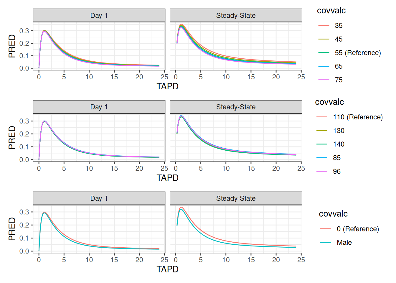
Simulation With Parameter Uncertainty

We need to run the simulations repeatedly, sampling parameters based on uncertainty estimates. This can be done in various ways. First of all, one must choose between non-parametric and parametric sampling. Non-parameteric sampling is typically based on a bootstrap, and the parametetric sampling is often based on a successfull $COVARIANCE step. NMsim has methods to do either type, and multiple methods are available for parametric sampling. The best source of information on these different methods is the ACOP2024 poster Simulation of clinical trial predictions with model uncertainty using NMsim by Sanaya Shroff and Philip Delff.

In this case we shall use parametric sampling, relying on a Nonmem $COVARIANCE step. Since in this case we are simulating typical subjects (random effects fixed at zero), we only need variability on the fixed effects (THETA’s). Multiple methods are available in NMsim to do this. We use NMsim_NWPRI - which automates simulation using the Nonmem NWPRI subroutine to sample the parameter sets. This simulation method excels in being fast to execute because it simulates all the parameter sets sequentially in one Nonmem run. It is important to run this with typical=TRUE. If between-subject variability is desired, please refer to NMsim-ParamUncertain.html.

simres.forest.nwpri <- NMsim(file.mod # path to NONMEM model
                            ,data=dt.sim.covs, # simulation dataset
                            ,name.sim="nwpri_forest" # output name suffix
                            ,method.sim=NMsim_NWPRI # sampling with NWPRI
                            ,subproblems=1000 ## number of parameter sets sampled
                            ,typical=TRUE # FALSE to include BSV
                            ,table.vars=cc(PRED,IPRED) # output table variables
                            ,seed.R=342 # seed for reproducibility
                             )

If you encounter issues with samples that do not run, consider whether any of your uncertainty estimates on THETA’s could lead to sampled THETA’s that could make the model be undefined. This would often be absorption parameters, clearences, volumes or any other strictly positive parameter which is estimated with poor precision. If this happens, you may want to go back and estimate that THETA on the log scale to make sure all sampled values will be positive.

Show example

A quick way to look for this is by combining parameter estimates (from the .ext file) and the automatic labeling of the parameters using NMdata::NMrelate().

NMdata::NMreadExt(file.mod,as.fun="data.table")[par.type=="THETA",.(RSE=se/value),by=.(par.name,FIX)] |>
    NMdata::mergeCheck(NMdata::NMrelate(file.mod,par.type="THETA",as.fun="data.table")[,.(par.name,code)],by="par.name",quiet=TRUE)

par.name	RSE	code
THETA(1)	0.0804007	LTVKA=THETA(1)
THETA(2)	0.0136327	LTVV2=THETA(2)
THETA(3)	0.0789812	LTVCL=THETA(3)
THETA(4)	0.0481949	LTVV3=THETA(4)
THETA(5)	0.0292952	LTVQ=THETA(5)
THETA(6)	0.4222300	AGEEFF=THETA(6)
THETA(7)	1.9160784	WEIGHTEFF=THETA(7)
THETA(8)	0.1041536	MALEEFF=THETA(8)

A large RSE is a potential issue for strictly positive parameters (RSE=0.25 for a parameter with a positive estimate corresponds to roughly 1/10,000 chance that a sample is negative). In this case, THETAs are estimated on log scale, and the covariate effects could be negative, so this model does not seem to have such issues.

Post processing

NMsim provides a function to do the post processing of the set of simulations setup by forestDefineCovs(). The key steps performed by this function are outlined below. Most importantly, it normalizes the exposures by the reference value for each sampled set of parameters. Then, it derives median and a confidence interval as quantiles in the simulated distribution.

The step required by the user is to define the functions to derive relevant exposure metrics. We will use AUC 0-24h and Cmax. We are using IPRED for the calculations. Notice, the simulation was run with typical=TRUE so PRED and IPRED should be the same. However, with depending on the Nonmem version, NWPRI works a little differently, and IPRED has to be used prior to Nonmem 7.6.0.

### Define exposure metrics
funs.exposure <- list(
    "Cmax"=function(x) max(x$IPRED)
   ,"AUC"=function(x) trapez(x$TIME,x$IPRED)
    ## ,"Concentration at 4 hours"=function(x) x$value[x$TAPD==4]
)

sum.uncertain <- forestSummarize(simres,
                                 funs.exposure = funs.exposure,
                                 by=cc(period),
                                 cover.ci=.95
                                 )

setDT(sum.uncertain)
sum.uncertain[covlabel=="Bodyweigt (kg)",covlabel:="Bodyweight (kg)"]

Plotting

We will use the R package coveffectsplot for plotting. coveffectsplot::forest_plot() requires certain column names so we adjust those first. An acceptance region such as the 80%-125% bio equivalence is included.

setDT(sum.uncertain)
setnames(sum.uncertain,
         cc(covvalf,predmm,predml,predmu,metric.var),
         cc(label,mid,lower,upper,paramname)
         )

sum.uncertain[,MEANVAL:=mid]
sum.uncertain[,covname:=covlabel]
nsig <- 3
sum.uncertain[,LABEL := sprintf("%s [%s - %s]",signif2(mid,nsig),signif2(lower,nsig),signif2(upper,nsig))]


descrip.legend <- "Reference (vertical line)\nClinically relevant limits 0.8-1.25 (colored area)"

### I don't know why forest_plot() needs this 
label_value <- function(x,... )x

fun.plot <- function(data,...){
    textsize <- 10
    forest1 <- forest_plot(
        data = data,
        facet_formula = "covlabel ~ paramname", 
        facet_scales = "free_y",
        facet_space = "free_y",
        xy_facet_text_bold = FALSE, 
        plot_table_ratio = 1.7, 
        table_text_size = 3,
        x_label_text_size = textsize,
        y_label_text_size = textsize, 
        x_facet_text_size = textsize, 
        y_facet_text_size = textsize,
        base_size=textsize,
        strip_placement = "outside",
        table_position = "right",
        legend_order = c("pointinterval", "ref", "area"),
        x_range = c(.5,1.5),
        ref_legend_text = descrip.legend,
        area_legend_text = descrip.legend,
        facet_switch = c("y"),
        legend_position="bottom",
        ...
    )
}

forest.day1 <- fun.plot(sum.uncertain[period=="Day 1"])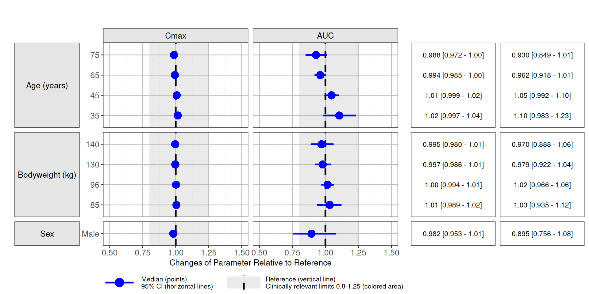

forest.ss <- fun.plot(sum.uncertain[period=="Steady-State"])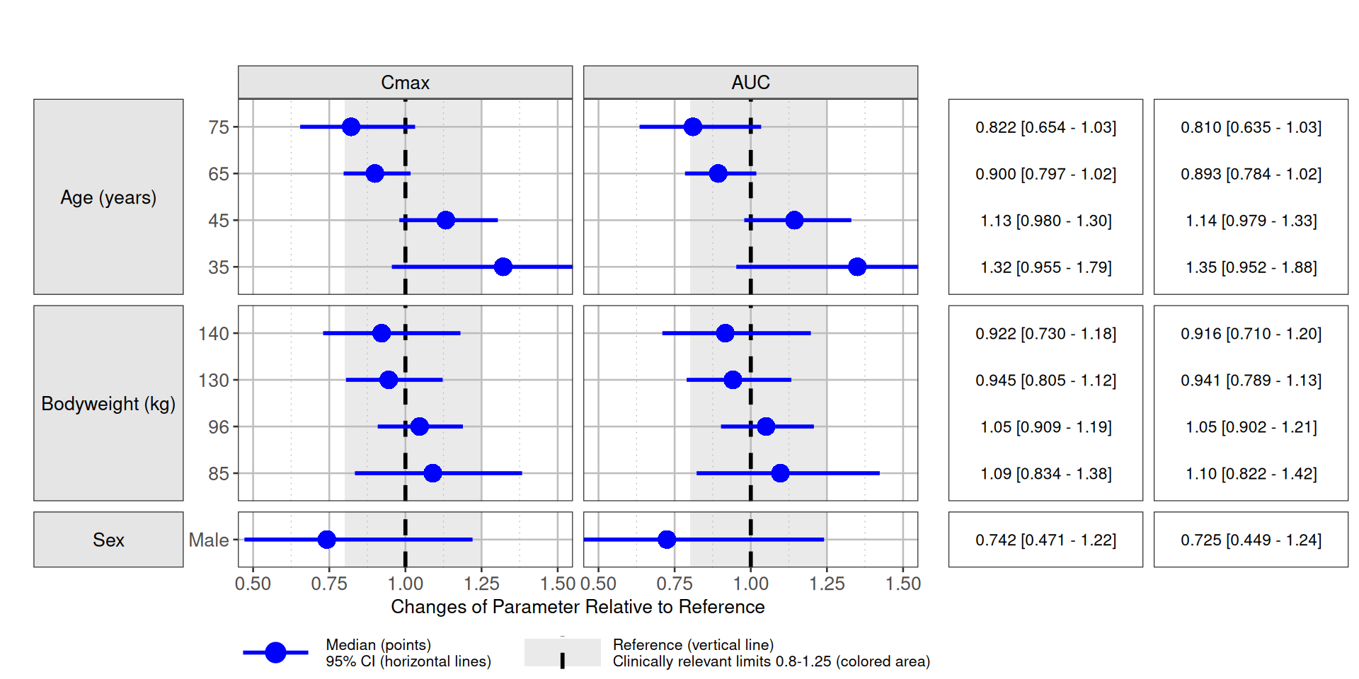

Simulation using multivariate normal distribution

We shall use the method provided by NMsim based on the multivariate normal distribution (mvrnorm). This method is selected because it is adequate for sampling THETA’s, it does not require additional software installed, other than Nonmem.

ext.mvrnorm <- samplePars(file.mod=file.mod,nsim=1000,method="mvrnorm",seed.R=6789)

simres.forest.mvrnorm <- NMsim(file.mod # path to NONMEM model
                              ,data=dt.sim.covs, # simulation dataset
                              ,name.sim="mvrnorm_forest" # output name suffix
                              ,method.sim=NMsim_VarCov # sampling with mvrnorm
                              ,ext=ext.mvrnorm
                              ,typical=TRUE # FALSE to include BSV
                              ,table.vars=cc(PRED,IPRED) # output table variables
                              ,seed.R=342 # seed for reproducibility
                              ,sge=TRUE # TRUE if submitting to a cluster
                              ,nc=1
                               )

Simulation using simpar for parameter sampling

ext.simpar <- samplePars(file.mod=file.mod,nsim=1000,method="simpar",seed.R=789)

simres.forest.simpar <- NMsim(file.mod # path to NONMEM model
                             ,data=dt.sim.covs, # simulation dataset
                             ,name.sim="simpar_forest" # output name suffix
                             ,method.sim=NMsim_VarCov # sampling with mvrnorm
                             ,ext=ext.simpar
                             ,typical=TRUE # FALSE to include BSV
                             ,table.vars=cc(PRED,IPRED) # output table variables
                             ,seed.R=342 # seed for reproducibility
                             ,sge=TRUE # TRUE if submitting to a cluster
                             ,nc=1
                              )

Simulation using bootstrap for parameter sampling

dir.bs <- "NMsim-forest-models/xgxr134_bs_N1000/m1"
exts.bs <- list.files(dir.bs,pattern=".+\\.ext$",recursive=T,full.names = TRUE)
ext.boot <- NMreadExt(exts.bs,as.fun="data.table")

simres.forest.boot <- NMsim(file.mod # path to NONMEM model
                           ,data=dt.sim.covs, # simulation dataset
                           ,name.sim="boot_forest" # output name suffix
                           ,method.sim=NMsim_VarCov # sampling with mvrnorm
                           ,ext=ext.boot
                           ,typical=TRUE # FALSE to include BSV
                           ,table.vars=cc(PRED,IPRED) # output table variables
                           ,seed.R=342 # seed for reproducibility
                           ,sge=TRUE # TRUE if submitting to a cluster
                           ,nc=1
                            )

Comparison of different simulation methods

The forest were simulated with all the methods mentioned above. As expected, the forest plots are very similar for NWPRI, mvrnorm, and simpar. This is expected because they all sample THETAs from the multivariate normal distribution. Among these, NMsim_NWPRI is the fasted to execute. A bootstrap may be desired or needed for a non-parametric approach. Remember that this is a very simple model, and similarities in the results based on the parametric models and bootstrap cannot be generalized based on this.

Collecting, Summarizing, and Plotting all Results

simres.forest.nwpri <- NMreadSim(c("simres-forest/xgxr134_nwpri_forest_MetaData.rds"),as.fun="data.table")
simres.forest.mvrnorm <- NMreadSim(c("simres-forest/xgxr134_mvrnorm_forest_MetaData.rds"),as.fun="data.table")
simres.forest.simpar <- NMreadSim(c("simres-forest/xgxr134_simpar_forest_MetaData.rds"),wait=TRUE,as.fun="data.table")
simres.forest.boot <- NMreadSim(c("simres-forest/xgxr134_boot_forest_MetaData.rds"),wait=T,as.fun="data.table")


simres.forest.all <- rbind(simres.forest.nwpri[,method:="NWPRI"],
                           simres.forest.mvrnorm[,method:="mvrnorm"],
                           simres.forest.boot[,method:="Bootstrap"]
                          ,simres.forest.simpar[,method:="Simpar"]
                          ,fill=T
                           )

### How many samples used with each method?
unique(simres.forest.all[,.(method,model.sim,NMREP)])[,.N,by=.(method)]

method	N
NWPRI	1000
mvrnorm	1000
Bootstrap	1000
Simpar	1000

sum.uncertain <- forestSummarize(simres.forest.all,
                                 funs.exposure = funs.exposure,
                                 by=cc(method,period),
                                 cover.ci=.95,
                                 as.fun="data.table"
                                 )

plot.compare <- ggplot(sum.uncertain[period=="Steady-State"],aes(predmm,covvalf,colour=method))+
    geom_rect(aes(xmin=.8,xmax=1.2,ymin=-Inf,ymax=Inf,colour=NULL),fill="grey85")+
    geom_rect(aes(xmin=predml,xmax=predmu,ymin=covvalf,ymax=covvalf),
              position=ggstance::position_dodgev(height=0.5))+
    geom_point(position=ggstance::position_dodgev(height=0.5))+
    facet_grid(covlabel~metric.var,scales="free_y",switch="y")+
    geom_vline(xintercept=1,linetype=2)+
    labs(y="",x="Relative Covariate Effect",colour="Simulation Method")+
    theme(legend.position="bottom")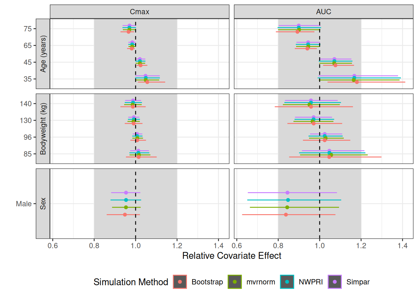

Post-processing step-by-step

We are including the code from the main steps in the post processing function, NMsim::forestSummarize(). It is important that the scientist understands that what the forest plots derived in this document represent is the relative effect of the covariate on the exposure metric. This is derived by NMsim::forestSummarize() as quantiles of the exposure relative to the reference subject. The confidence interval hence expresses the uncertainty on the covariate effect for a subject with other covariates at reference values.

Details on code used for summarizing forest plot statistics (click to show)

Notice, the code below consists of snippets from the NMsim::forestSummarize() function. The code is not intended to be used on its own.

### use only simulated samples
simres <- as.data.table(data)[EVID==2]


### summarizing exposure metrics for each subject in each model,
### each combination of covariates
resp.model <- simres[,lapply(funs.exposure,function(f)f(.SD)),
                     by=c(allby,modelby,"ID")]

### the exposure metrics in long format.
mvars <- names(funs.exposure)
resp.model.l <- melt(resp.model,measure.vars=mvars,variable.name="metric.var",value.name="metric.val")


## deriving median by model and time to have a single value per
## model This is only relevant in case multiple subjects are
## simulated by each model. 
sum.res.model <- resp.model.l[
   ,.(predm=median(metric.val))
   ,by=c(modelby,allby,"metric.var")
]

### making reference value a column rather than rows. 
## column with refrence exposure value is called val.exp.ref

### summarize distribution of ratio to ref across parameter samples/models
sum.uncertain <- sum.res.model[
   ,setNames(as.list(quantile(predm/val.exp.ref,probs=c((1-cover.ci)/2,.5,1-(1-cover.ci)/2))),
             c("predml","predmm","predmu"))
   ,by=c(allby,"metric.var")]

Philip Delff, Boris Grinshpun

May 06, 2025